POLYGON PLANARIZATION

Last week I had a great conversation with someone in the Houdini discord chat group about an interesting problem. He had a surface made up of quads and wanted to “planarize” the polygons in order to build a large physical model from it. He told me that he usually uses Grasshopper and Kangaroo for this but was wondering if it’s also doable in Houdini. Well, I don’t know Kangaroo very well but as far as I know it’s basically a particle-spring based solver. It uses a force based approach which works quite well for many different problems such as planarizing a polygonal mesh. (This isn’t true any more! Daniel wrote me in the comments below that Kangaroo is using a projective solver since 2014). Pretty much the same, of course, could be done in Houdini. By using a “planarization force” together with constraints in the grainSolver it’s easy to replicate such a system. Instead of using grains it’s also possible with wires. Most probably they’re not as stable as grains but nevertheless it should do the job. If we like we could also build our own force based solver. Implementing verlet integration in a solverSop is easy and apart from that there’s the gasIntegrator microsolver which we can use in DOPs for that purpose. However, to get a stable system it’s important to choose the right step size for the integration. If it’s too large the system explodes and if it’s to small it takes forever to find its equilibrium. Of course, higher order integrators like Runge Kutta are minimizing this problem and generally they are quite stable. The same is true for the position based approach of grains but the problem still remains, at least to some degree.
Anyway, it’s an interesting problem and even though it’s typically not too hard to solve it could become quite tricky depending on the geometry. The hard part is not so much to obtain planar polygons but to stay as close as possible to the original mesh. In the worst case we might end up with an entirely flat mesh what’s clearly not the intended result. The reason might be, for example, that the mesh describing the surface has an unfavourable structure. And sometimes it’s simply not possible because not every surface can be made up of planar polygons except triangles.
During our chat I remembered that there was a thread on OdForce about pretty much the same topic. Someone had a saddle-shaped surface for which he computed the dual mesh and subsequently wanted to make the resulting hexagons planar. At the same time the boundary points of the surface should keep their original position. Well, even though a saddle surface seems to be rather simple, it is not and I think this is a good example to highlight some of the problems we might run into when we’re trying to planarize polygons.

But first let’s take one step back and start simple. Instead of using hexagons let’s assume it is a quad mesh. One way to tackle this problem is to use a force based approach similar to what Kangaroo/Grasshopper is doing. We need to set up a number of forces and run the system until it reaches equilibrium. To calculate the “planarization-force” we could, for instance, project the polygon points onto the plane defined by center and normal. Or we compute the diagonals and check their distance to each other. To preserve the mesh structure we can rely on edges and diagonals as spring forces. Additionally we need to keep the points of the boundary at their position. The key point, however, is to adjust the weighting between all these forces to finally get the result we were looking for. Usually there is no way to find a solution satisfying all the objectives and hence the result is highly depending on how we balance the forces. As said above, such an approach is easy to set up and it works quite well under most circumstances. However, for a number of reasons I thought it might be better to take a slightly different approach. Instead of using a force based system I used a method which is conceptually somewhat similar to the “As Rigid As Possible Surface Modelling” approach. Intuitively it’s easy to understand and works basically in the following way:

For every polygon of the mesh, the planar counterpart is computed and then fitted to the original poly in the least squares sense. For our specific “planarization problem” we could also just project the points onto the tangent plane but in general we may want to rely on rigid shape matching to find the best fitting orientation. This could be done easily in VEX by using polardecomp() or by using Numpy. Even though polar decomposition in VEX is faster I tend to use Numpy’s SVD algorithm since it doesn’t have problems with flat axis aligned polys. Of course, we could make our matrix positive by adding a very small value but this might lead to other problems instead. For a high number of polygons it’s a good idea to implement a simplified SVD algorithm in VEX which doesn’t have such problems but in most cases Numpy should be fast enough. But let’s not get off the track and back to the planarization problem.
After the “planarization” step is applied to each polygon the mesh is obviously torn apart. What we need to do next is to reconstruct the mesh in the least squares sense based on the planar polygons. In other words, we need to set up and solve a linear system. If we repeat these steps iteratively a number of times the system finally converges to the solution we are looking for. The result is the mesh made up of planar polygons. So, the process boiles down to the following threes steps:

• Fit planar polygon to original polygon in the least squares sense
• Reconstruct mesh based on planar polygons in the least squares sense
• Repeat until system converges

Of course, we also need to implement all the other constraints too, such as fixed boundary points, mesh structure preservation and so on. In the example below, the four corner points are fixed at their position all the other points are allowed to move in all directions. In my tests the algorithms works quite well and is also relatively fast. For the mesh shown below it needs about 175 iterations and converges in about 280 ms on my rather old laptop.

Original mesh

Planarized mesh

Deviation to the original surface

Planarization

Original polygons

Planar polygons

Planarization

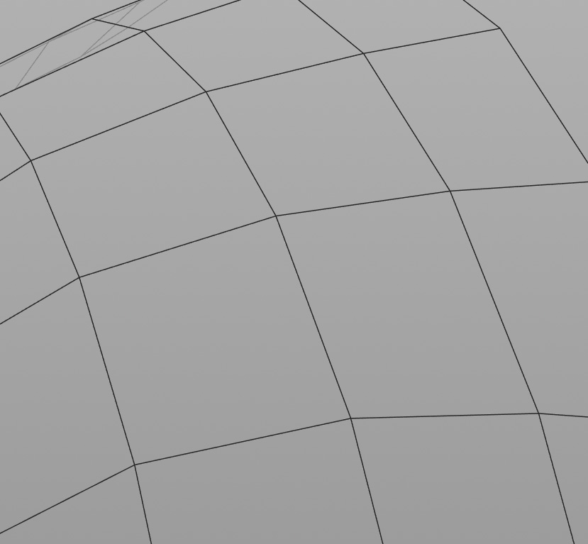
But now let’s go back to the example file from OdForce. The original question was how to obtain planar hexagons while retaining the overall shape of the mesh. Additionally, even though it’s not mentioned in the post, we may want to keep the mesh structure intact. In other words, the polygons should stay connected. Well, this sounds easier than it is. It is indeed possible but we might end up with unwanted results. The problem is that the saddle-shaped surface has negative gaussian curvature and hence it can’t be approximated by convex hexagonal polygons. However, if we allow non-convex polygons it’s doable although the deviation to the original shape is rather large. This is clearly visible in image 2 and 3 below. If we additionally allow for open edges the overall shape is preserved very well (image 4). However, this is just the case for hexagonal polygons and won’t work for quads in the same way. So let’s take a look what happens if we choose four-sided instead of six-sided polygons.
(Side note: For computing planar hexagonal meshes it’s most probably more efficient to rebuild the mesh instead of planarizing it’s polygons but that’s maybe a topic for another blog post)

Original non-planar hexagonal polygons

Planar non-convex polygons with open edges

Planar non-convex polygons with connected edges

Planar non-convex polygons with connected edges

Convex non-planar hexagonal polygons

Non-convex planar hexagonal polygons

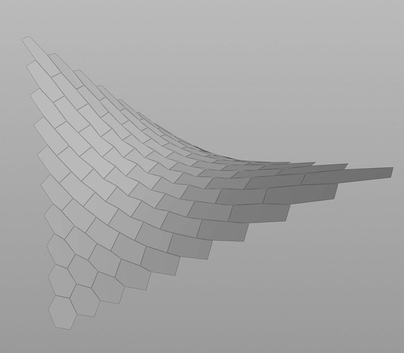
Using the planarization algorithm on the quad mesh results in a completely flat surface which is clearly not what we want. But how could this happen? Well, the simple reason is that it’s just not possible to obtain planar AND connected polygons based on our initial mesh without getting large deviations in the overall shape. This is clearly visible in the images below. Picture 1 is the original mesh made up of non-planar polygons. Picture 2 shows the result of the planarization with fixed corner points and picture 3 is the planarized poly mesh without any additional constraints.

Original mesh

Planarized mesh with fixed corner points

Planarized mesh

So what can we do to get a better result? The answer is simple. We need to provide a better starting point for the algorithm. In other words, we need to remesh the surface. The most natural way to remesh a surface is based on it’s principal curvature direction. By integrating the fields, for example, we could extract a conjugate curve network which we then use to construct the mesh. Such a curvature aligned mesh is exactly what we need since it’s quads are naturally close to planar. For simple geometries this is not too hard to implement and the resulting mesh is a perfect starting point for the subsequent planarization algorithm. In the case of our saddle-shaped surface it’s even better because we don’t need to do any planarization at all. The new curvature aligned mesh is already composed of fully planar polygons.

Curvature based cross field

Conjugate curves

Curvature aligned mesh

For some related reading:
R. Poranne, E. Ovreiu, C. Gotsman: Interactive Planarization and Optimization of 3D Meshes
S. Bouaziz, S. Martin, T. Liu, L. Kavan, M.Pauly: Projective Dynamics: Fusing Constraint Projections for Fast Simulations
W. Wang, Y. Liu: A Note on Planar Hexagonal Meshes
W. Wang, Y. Liu, B Chan, R. Ling, F. Sun: Hexagonal Meshes with Planar Faces