SHAPE SIMILARITY

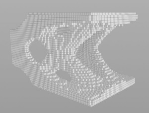
This is a follow-up to this blog post where I had written about various spatial metrics, but didn’t go into detail about how they are calculated and what they mean. This post is now the first of several to follow that will be about just these things.

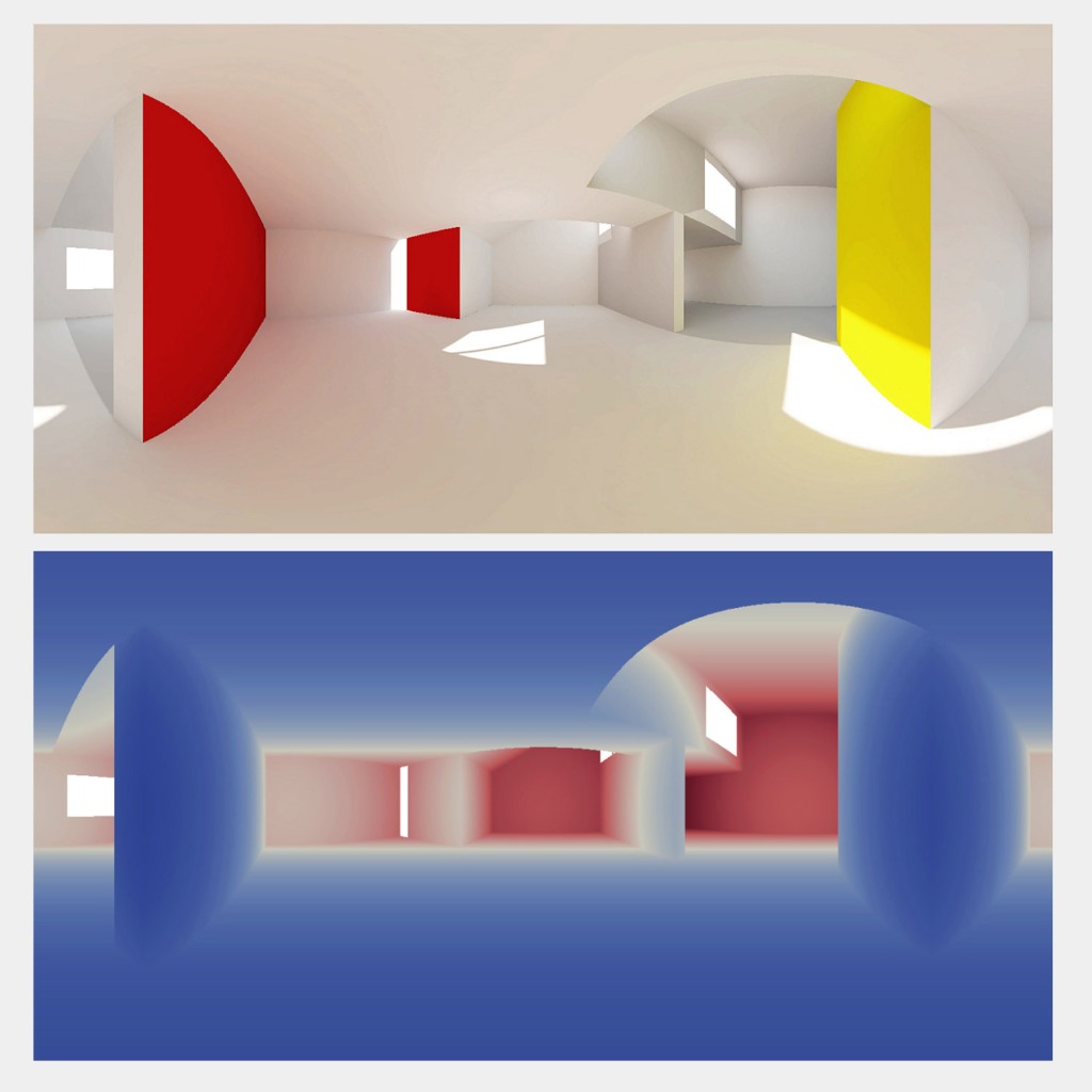
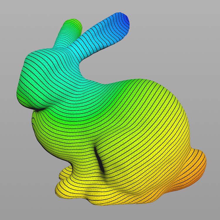
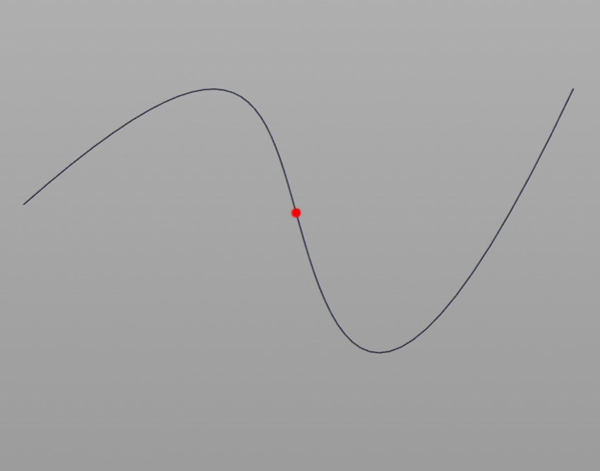
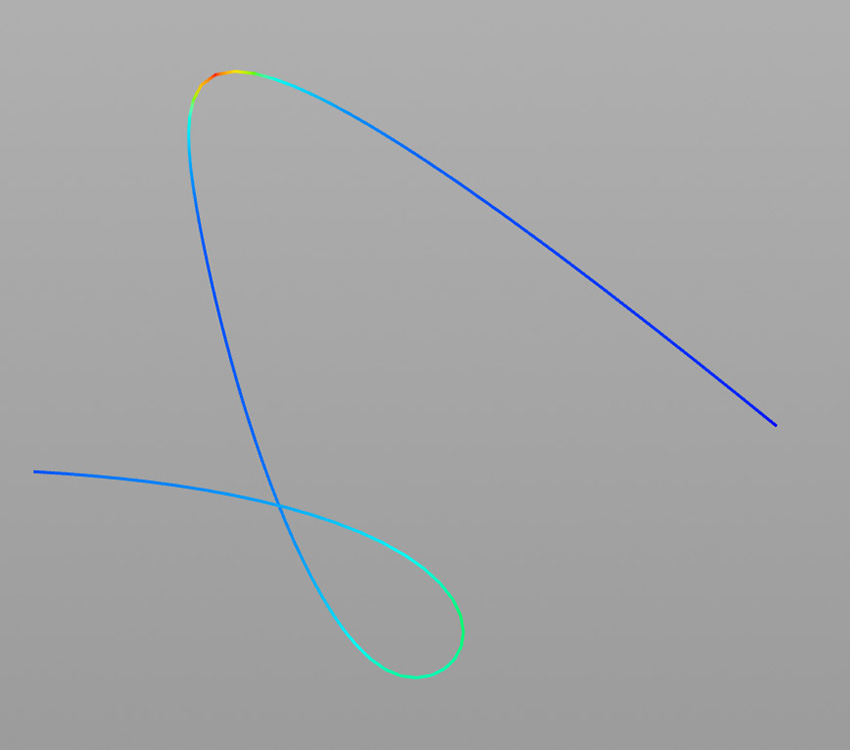
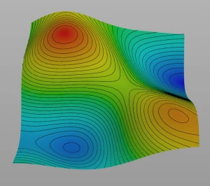
So let’s start simple with the measure of similarity. But before that, some background on why we want to calculate it in the first place. Typically, an isovist describes local spatial properties. However, since (human) perception is strongly related to motion and locomotion, it makes sense to capture it in terms of relational or semi-global measures that account for motion to a certain degree; as an example, we might want to know the change in visible space relative to a change in position. One such metric is the measure of revelation. Revelation was introduced by Franz and Wiener and later further developed and refined by Dalton in his PhD thesis. It basically measures how much “new space” is revealed or lost as a person moves through space. It is calculated by taking the difference between the area of the current isovist and the mean area of adjacent (and visible) isovists. An alternative definition is to consider all isovists visible from the starting isovist, or more precisely, from the current position. Thus, the measure of revelation is conceptually somewhat related to the famous Laplacian (which I have written about many times on this blog in the past …).

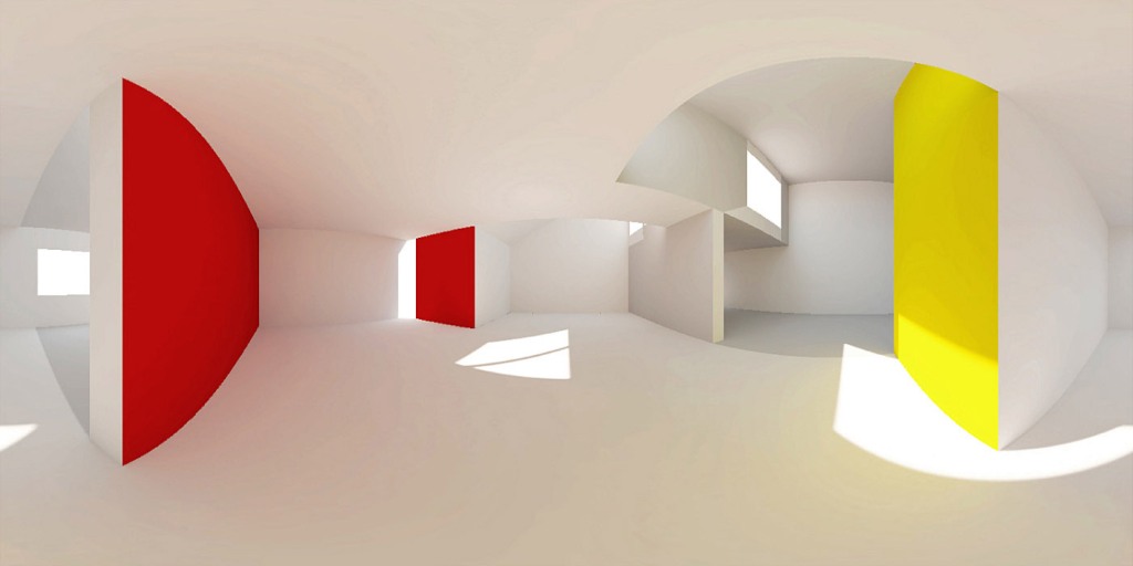
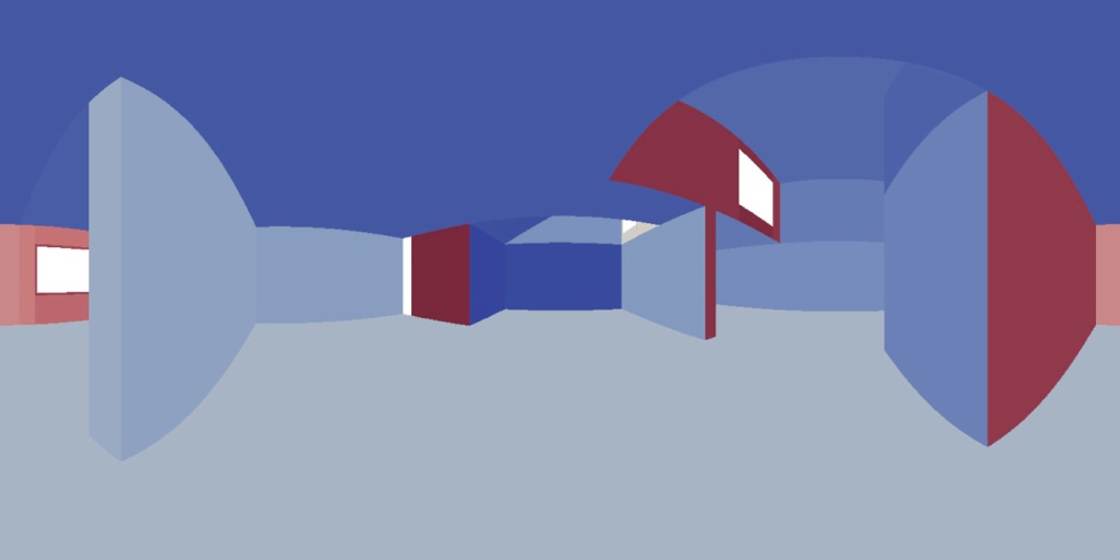
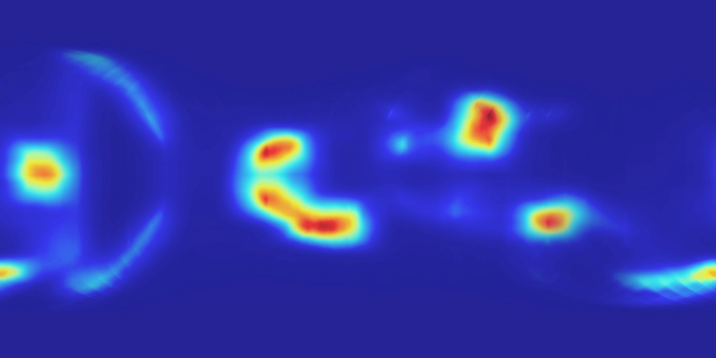
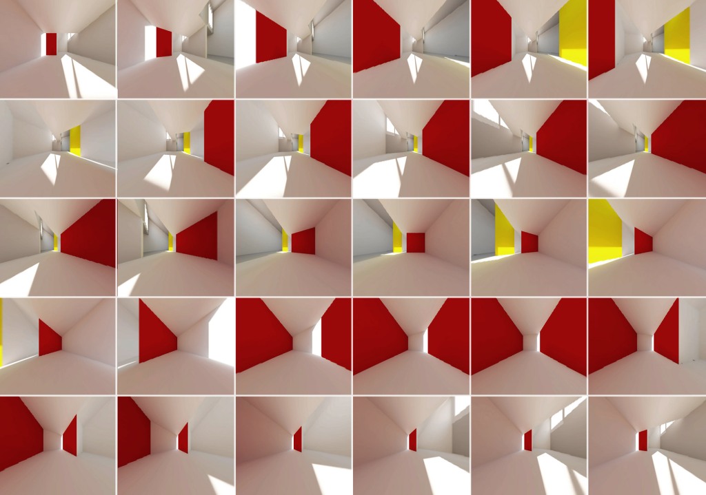
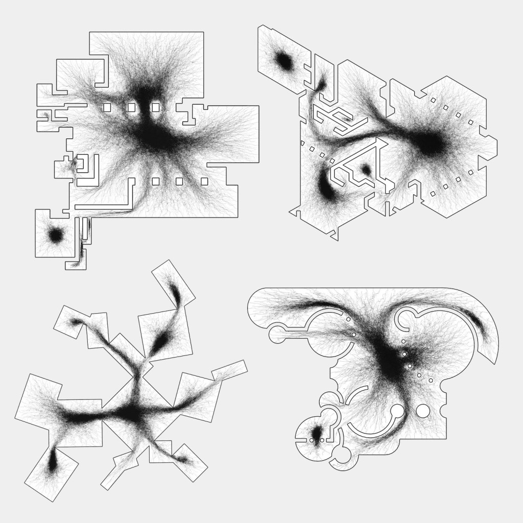
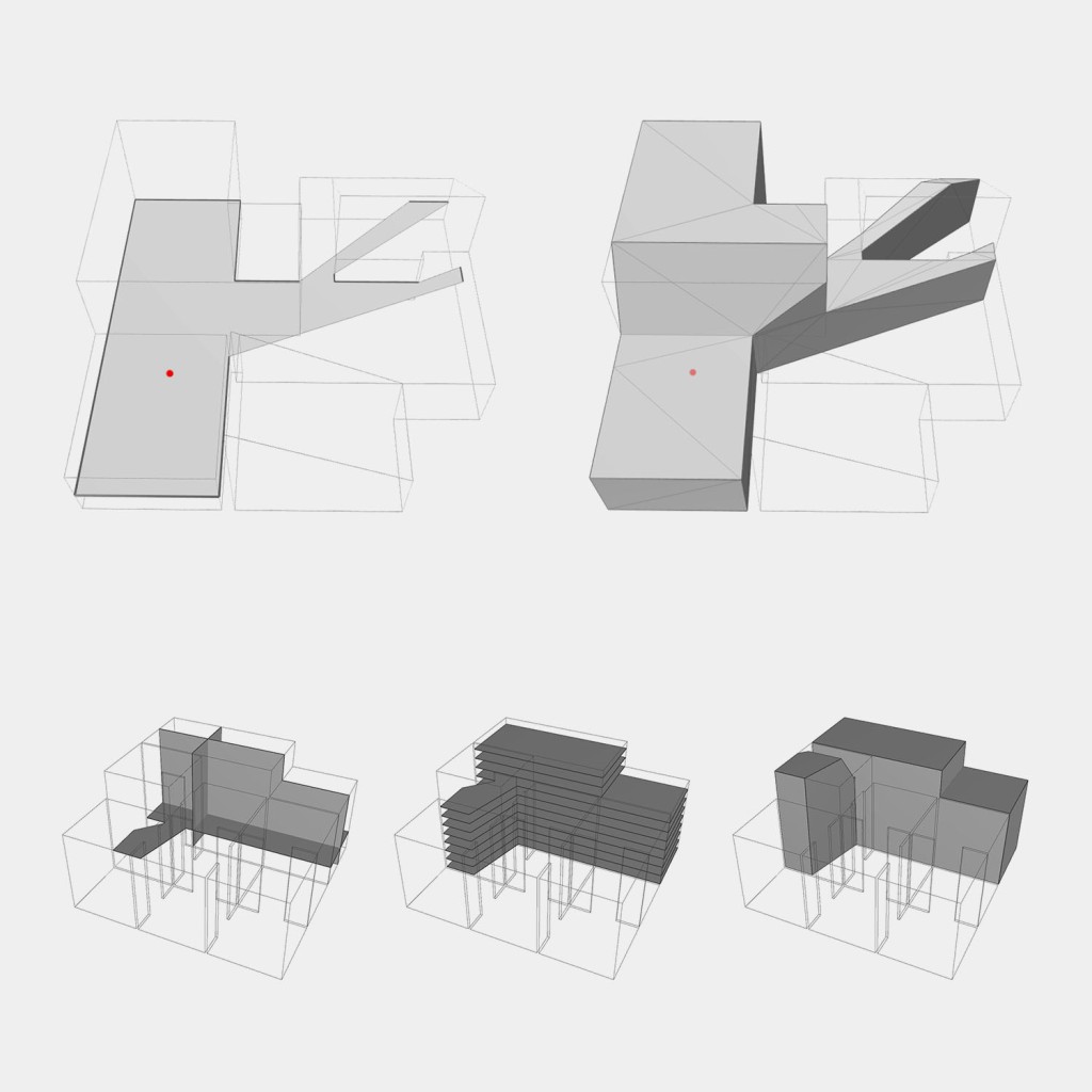
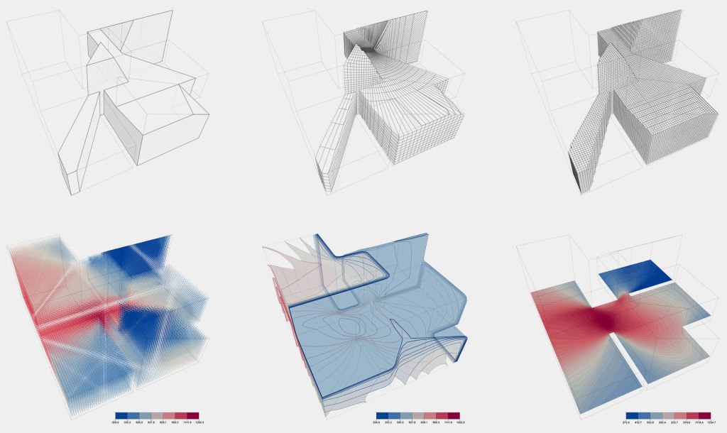
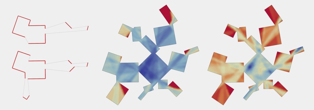
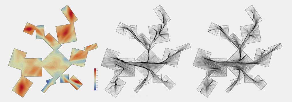
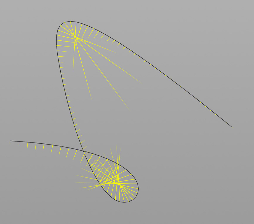
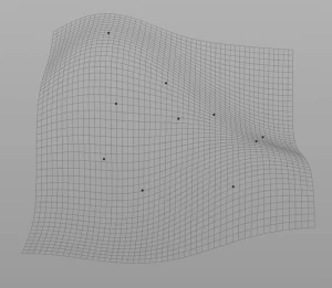
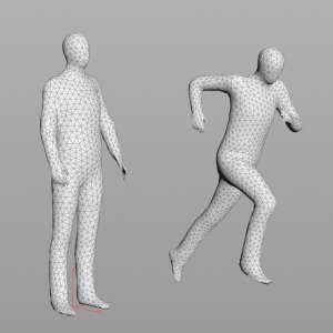
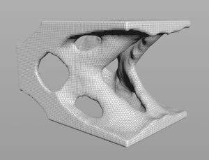
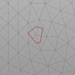
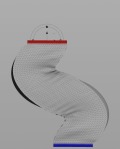
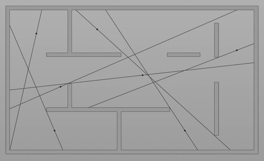
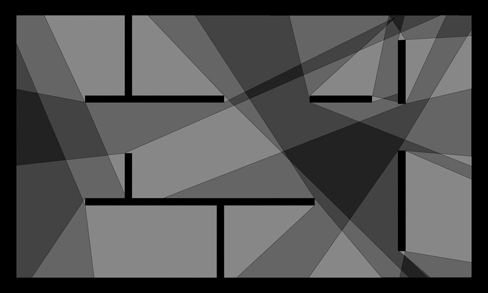
Now, to make it a little less abstract, let’s look at a simple example. An isovist is a geometric representation of visible space, relative to a particular position. Although geometrically it is a closed polygonal/polyhedral shape, not all boundary edges/polygons exist in reality. These “non-existent” boundary edges are simply extensions of the lines of sight and are called occluding edges. However, they do not match up with the surfaces of the “real” environment. Edges that match actual boundaries of the environment are called solid edges. The number and length, as well as their ratio, are very important properties as they capture various features of the environment from which the isovist is generated. Slightly simplified, we can say that the more occluding edges an isovist has and the longer these edges are, the more space will potentially be revealed when moving from one position to another. As various research studies have shown,this measure is closely related to the way people navigate and move around in spaces.

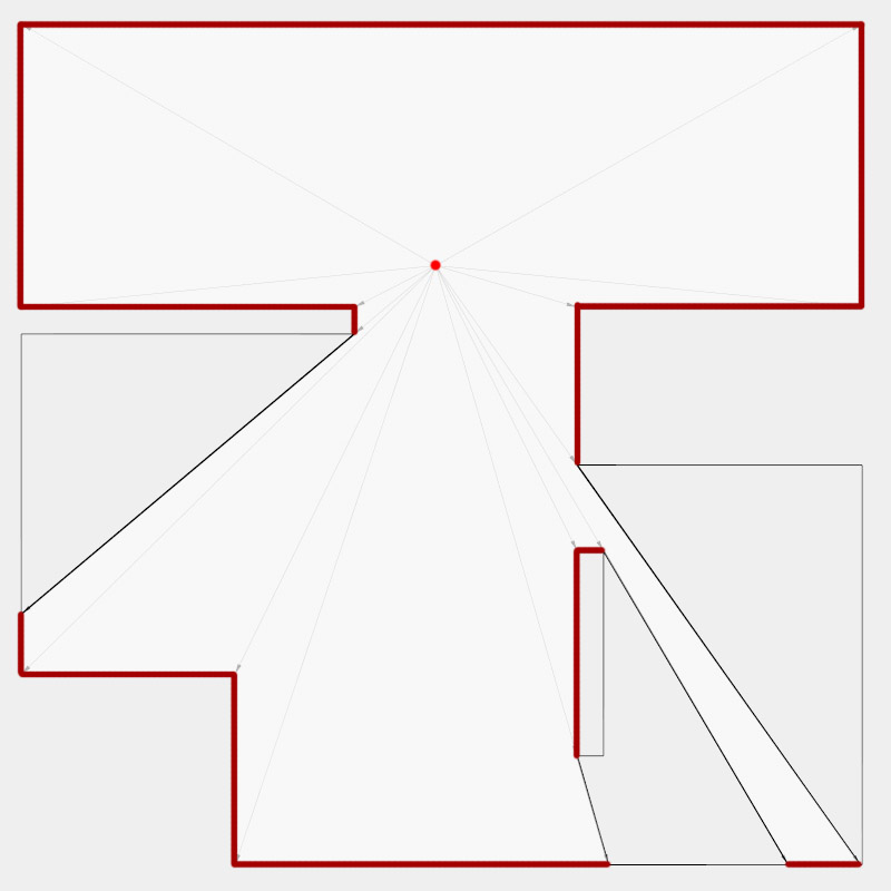
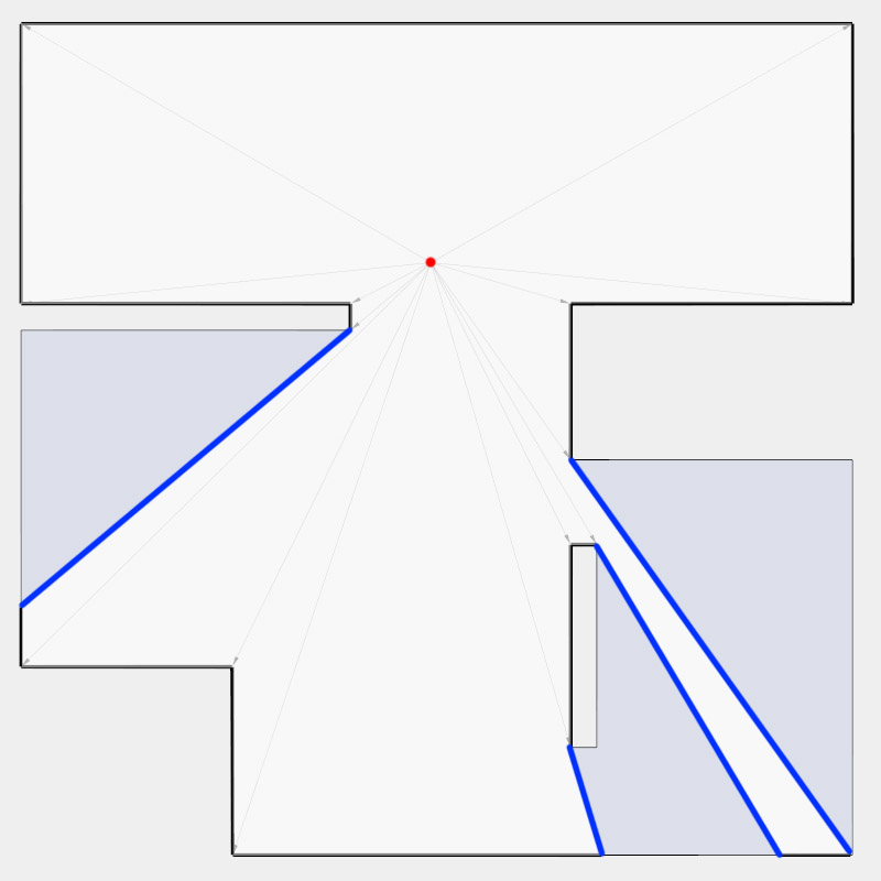
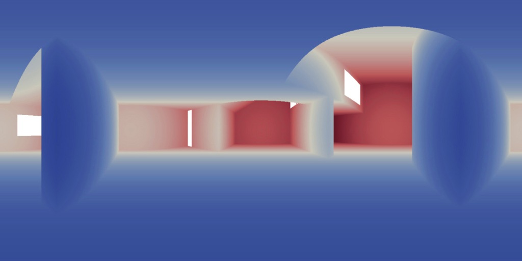
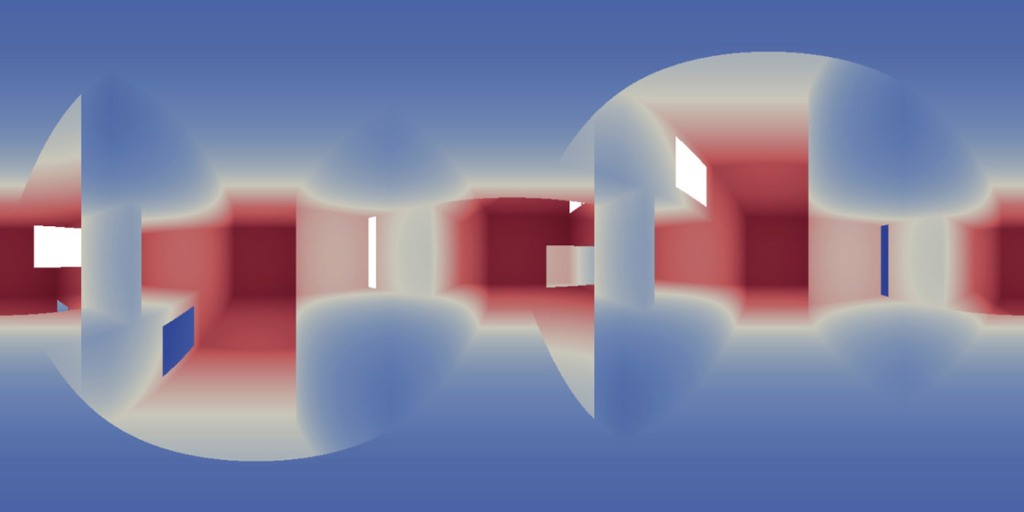
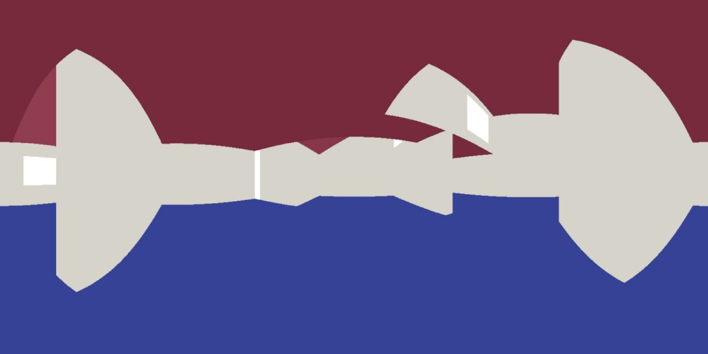
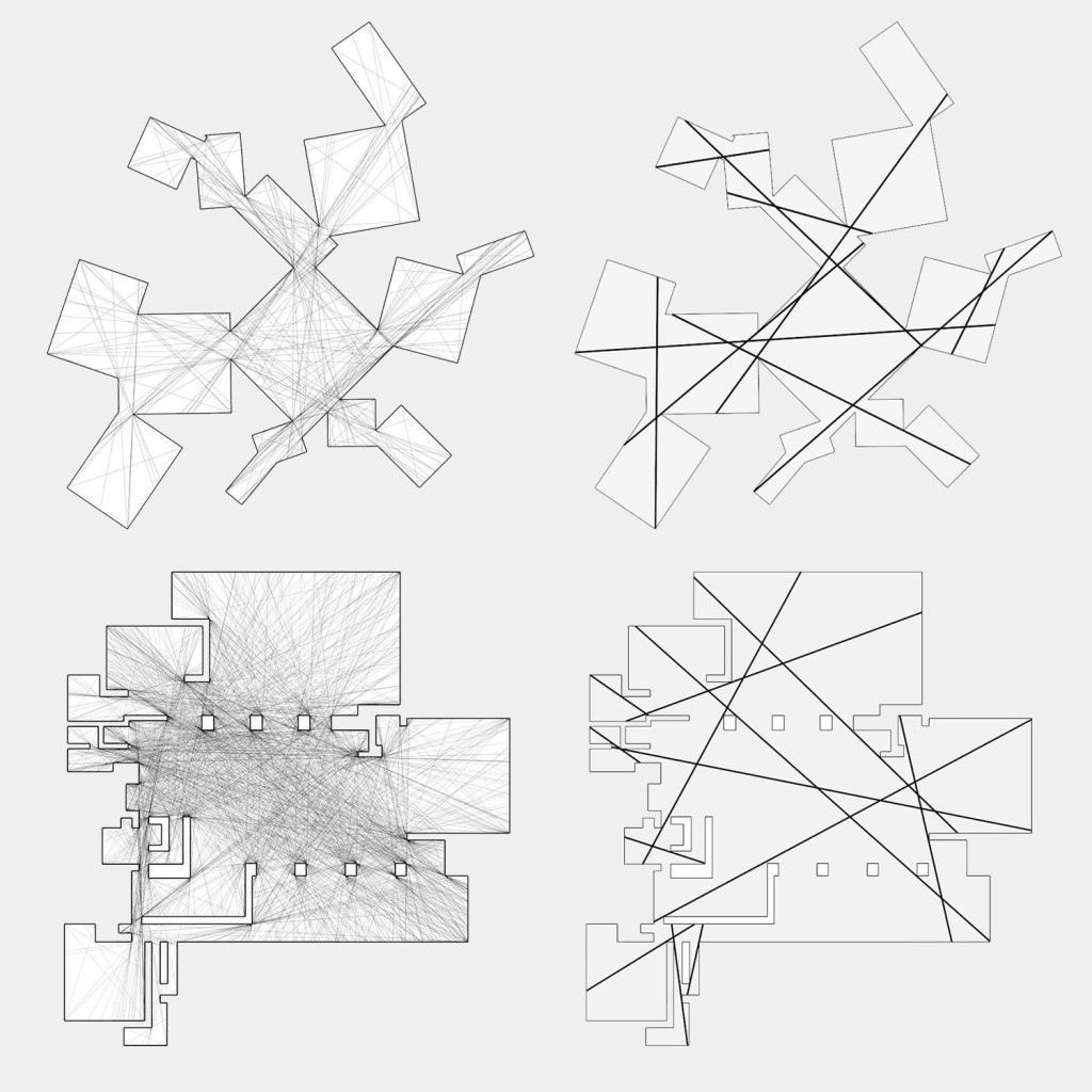
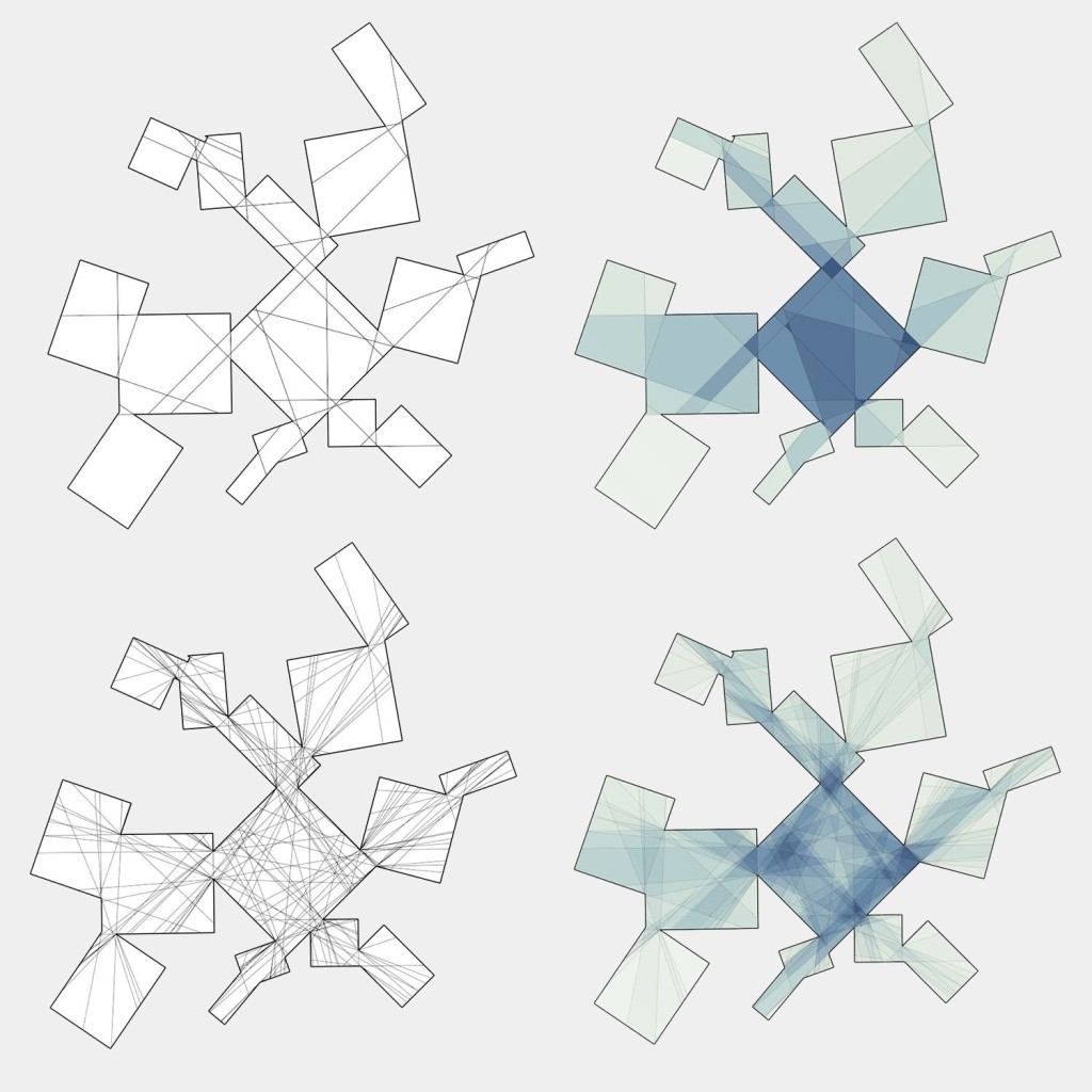
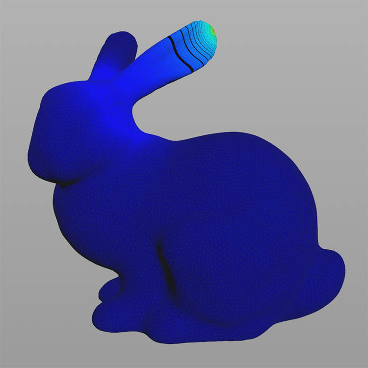
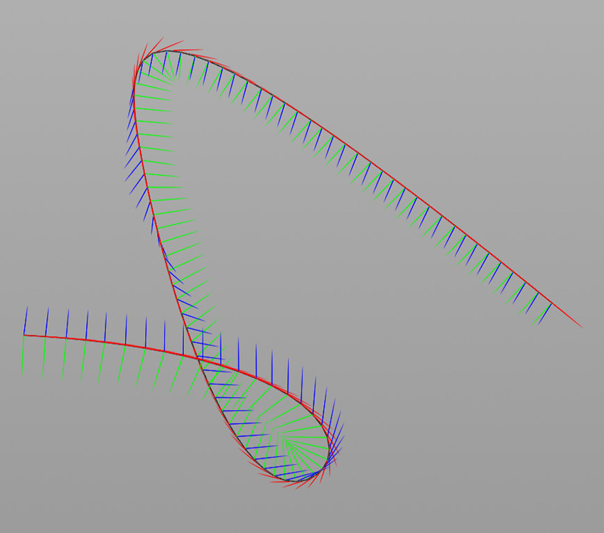
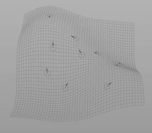
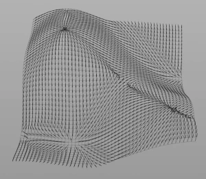
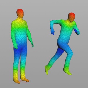
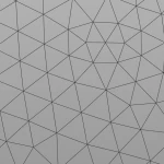
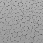
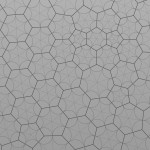
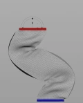
Two images on the right: Isovist polygons for two different locations. The thick red lines represent solid edges; the thinner black lines are occluding edges. Image on the right: The thick blue lines are occluding edges; the bluish color represents regions that could potentially be revealed by changing position.

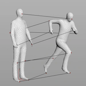
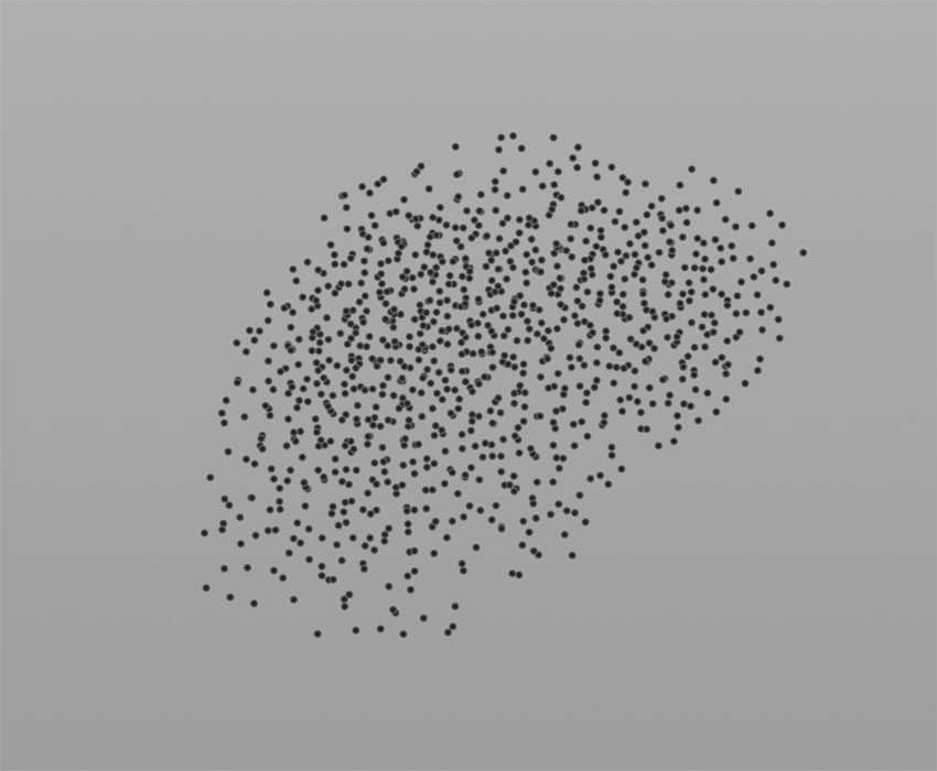
But now back to our similarity measure: Instead of considering only the change in area, we can also consider how much an isovist polygon/polyhedron changes geometrically in terms of its shape. And to do that, we need a way to quantify that change. The most obvious method, of course, is to sum the distances between each point of an isovist and the corresponding point of another isovist. After normalizing the total distance difference by the area of the isovists, we get what is certainly a valuable measure of how similar two shapes are. An even simpler way is to measure the difference between isovists by their radial distances. However, this method only works if the isovists have the same number and order of points, which might not be the case for two reasons: (1) we compute exact isovists (more on this here) or, (2) we compute the similarity measure only between solid edges of isovists. Fortunately, the similarity of shapes is an important property in computational geometry, and hence there are many papers by different authors providing different approaches to address this problem. The method I chose to implement is based on a paper by Belongie, Malik, and Puzicha and is a slightly modified version of their Shape Context Descriptor. This method is quite robust, fairly insensitive for noise, works in two and three dimensions, and since it’s essentially a statistical approach, it works with different numbers and orders of points. And last but not least, it can be easily implemented in OpenCL.

Basically it works as follows:

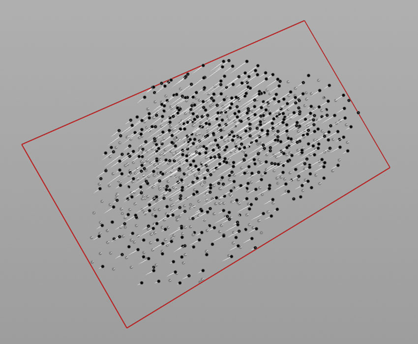
Calculate the (euclidean) distance from each point to every other point of an isovist
Calculate the mean distance and normalize all distances by this value (this results in distance values between 0.0 and 2.0)
Calculate the angle to all points
Shift the angles into the range of 0.0 – 2pi
Compute a distance histogram based on a logarithmic scale between 0.0 and 2.0
Count the number of distances in each bin
Compute an angle histogram based on a linear scale between 0.0 and 2pi
Count the number of angles in each bins
Combine both histograms to get the local shape context descriptor
Repeat the steps above for each point
And finally compare two shapes by calculating the “difference” between the local descriptor from each point on one shape to every point on the other shape

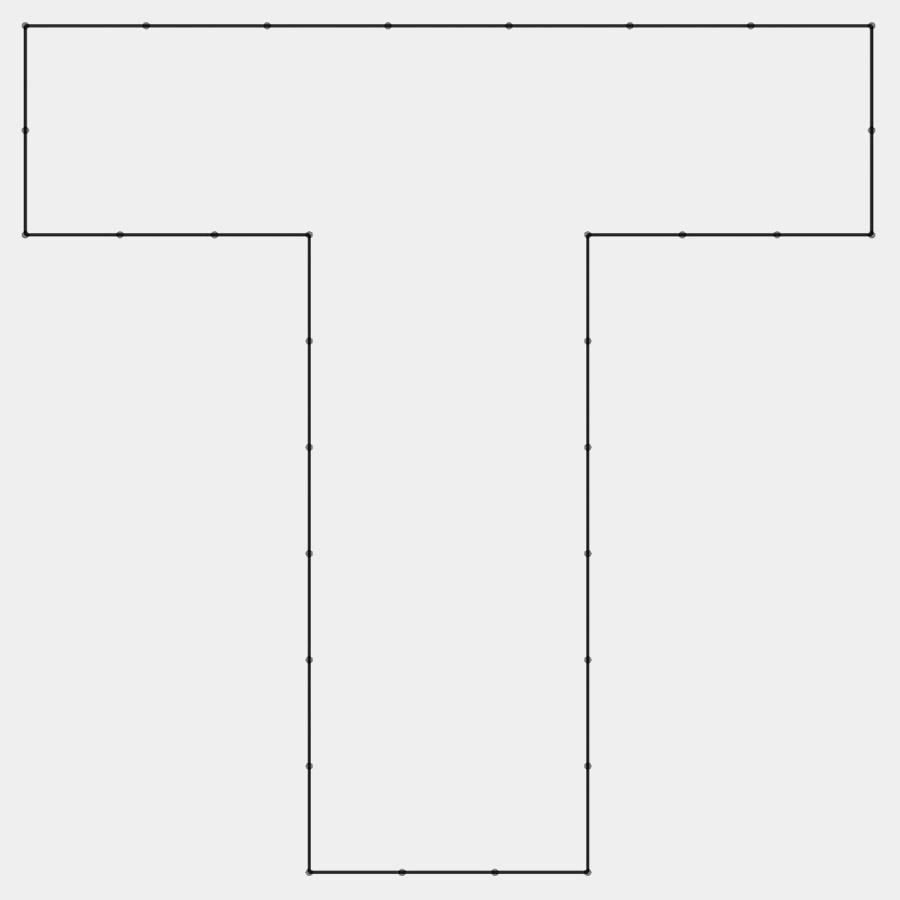
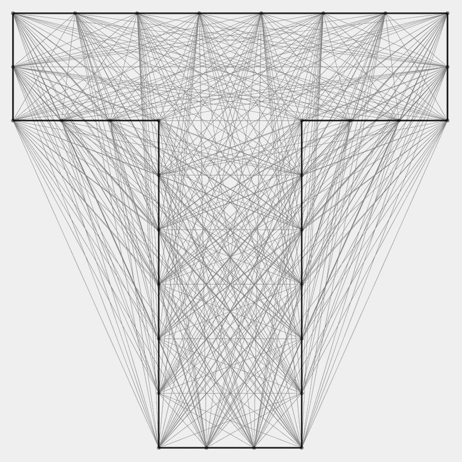
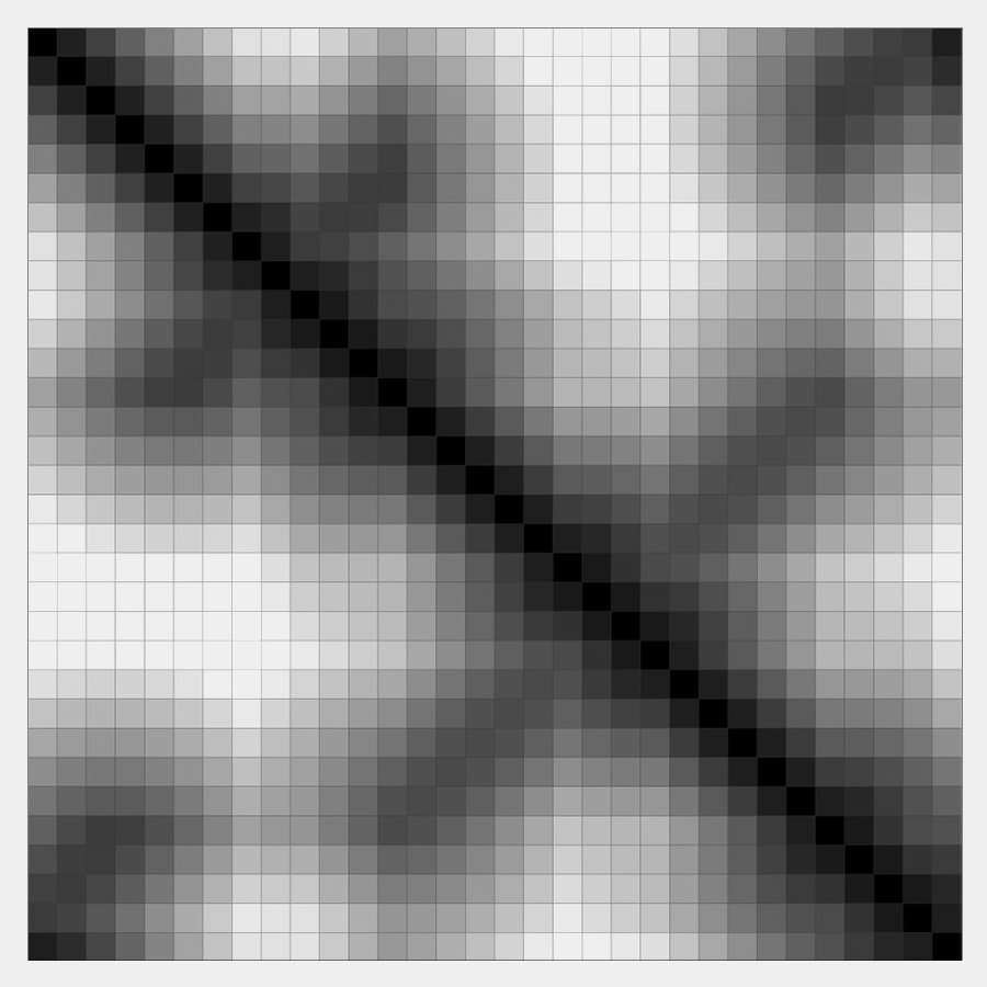
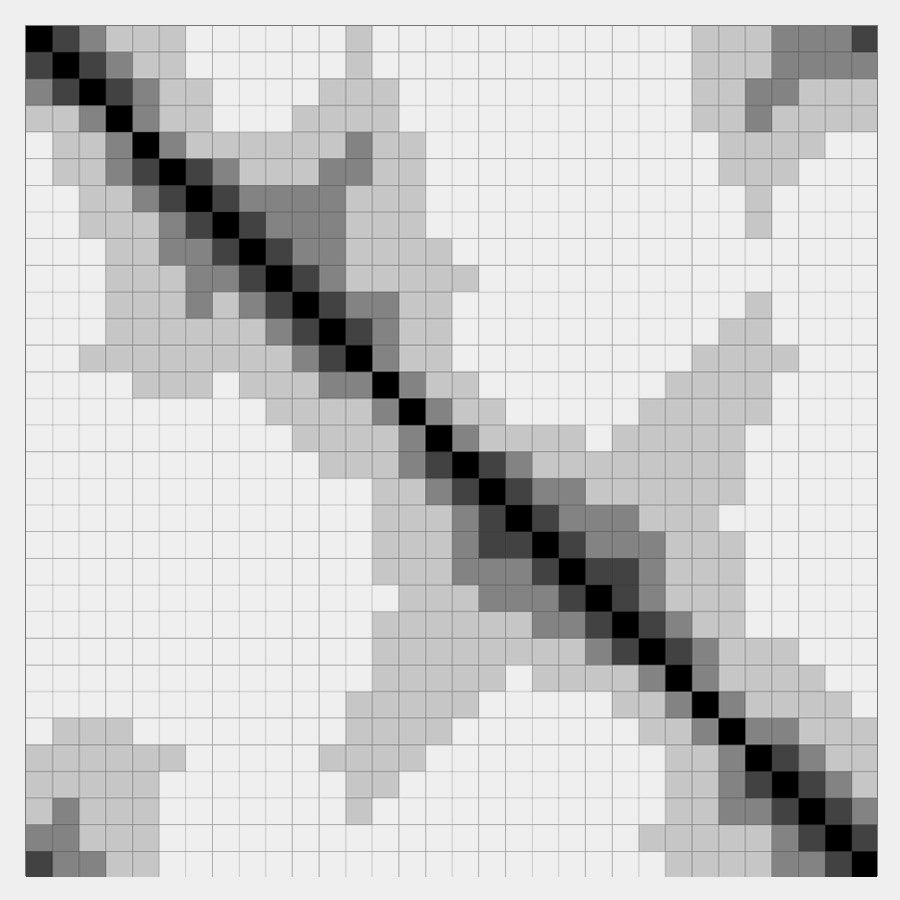
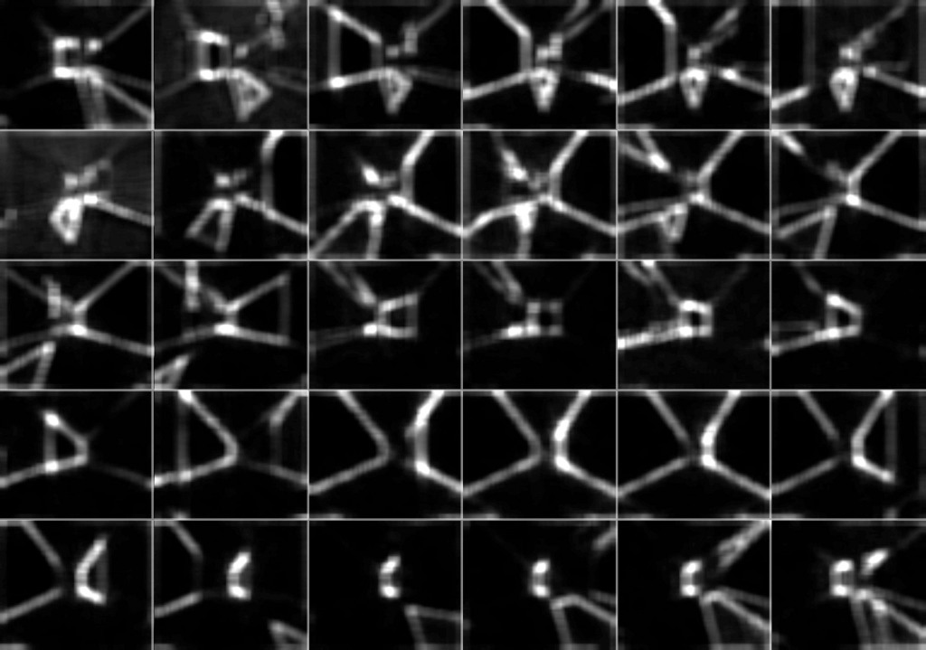
Distance histogram computation from left to right: (1) polygonal shape; (2) euclidean distance between all points; (3) distance matrix; (4) bin matrix for distance histogram (number of bins = 5)

In the same way that we computed the distance histogram, we can compute the angle histogram. Combining the two, we finally get the shape context descriptor for each point, which captures the local distribution of points relative to each point on the shape. However, instead of building it in matrix form, we store it as a flat array, so that it can be processed without problems by OpenCL.

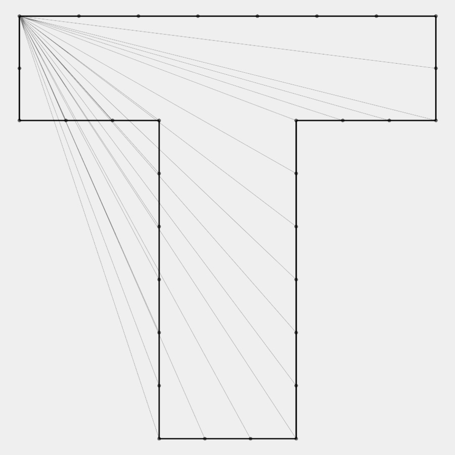
Right: Distance and angle from one point to every other point on the shape. Left: Shape context descriptor for one point.

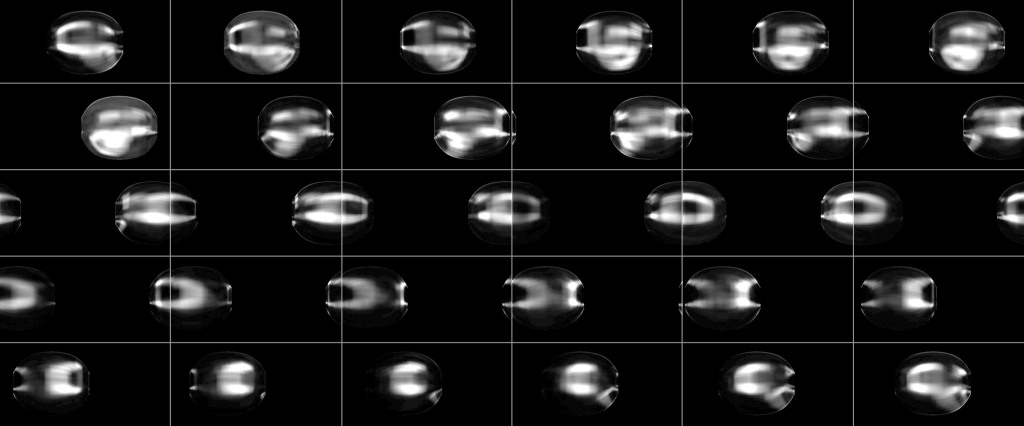
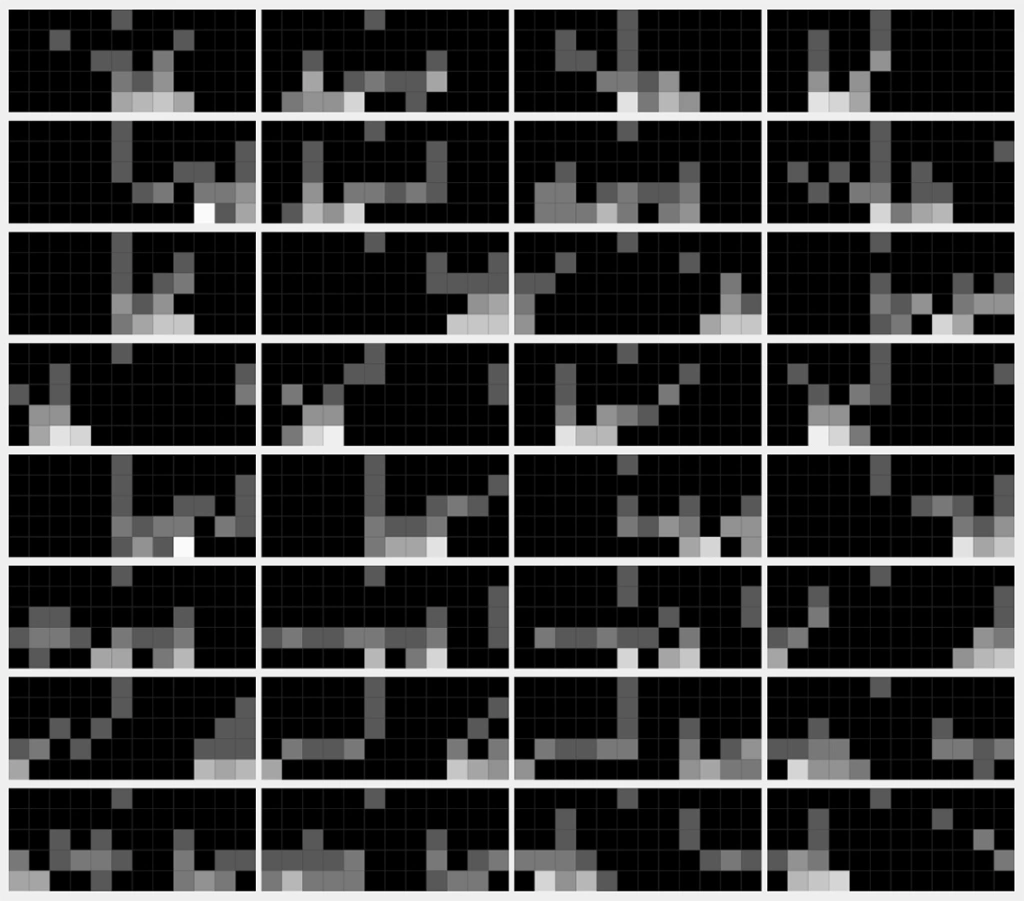
To calculate the similarity of shapes, we would normally calculate the difference between each point on one shape to each point on another shape. However, for performance reasons, I combine all local descriptors per point into one global descriptor per shape/isovist. Computing the similarity between thousands of shapes/isovists is therefore much faster, though less accurate. However, for my purpose, the result is still accurate enough.

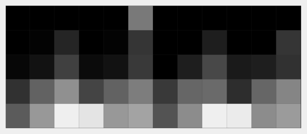
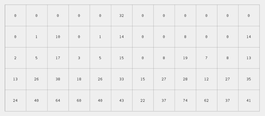
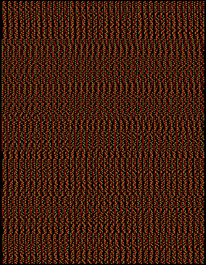
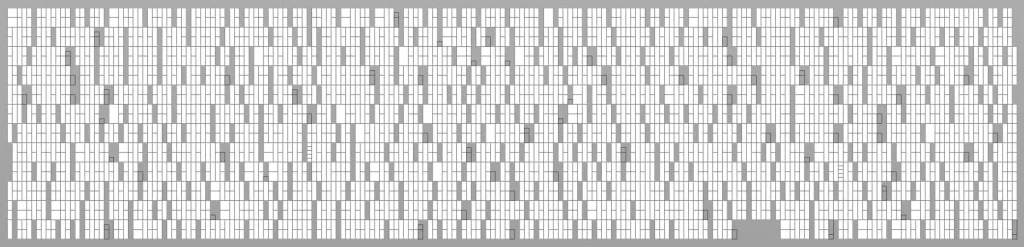
Combined per shape descriptor in matrix form (images at the top) and as flat array (image at the bottom). Number of bins for the distance histogram is 5, for the angle histogram 12.

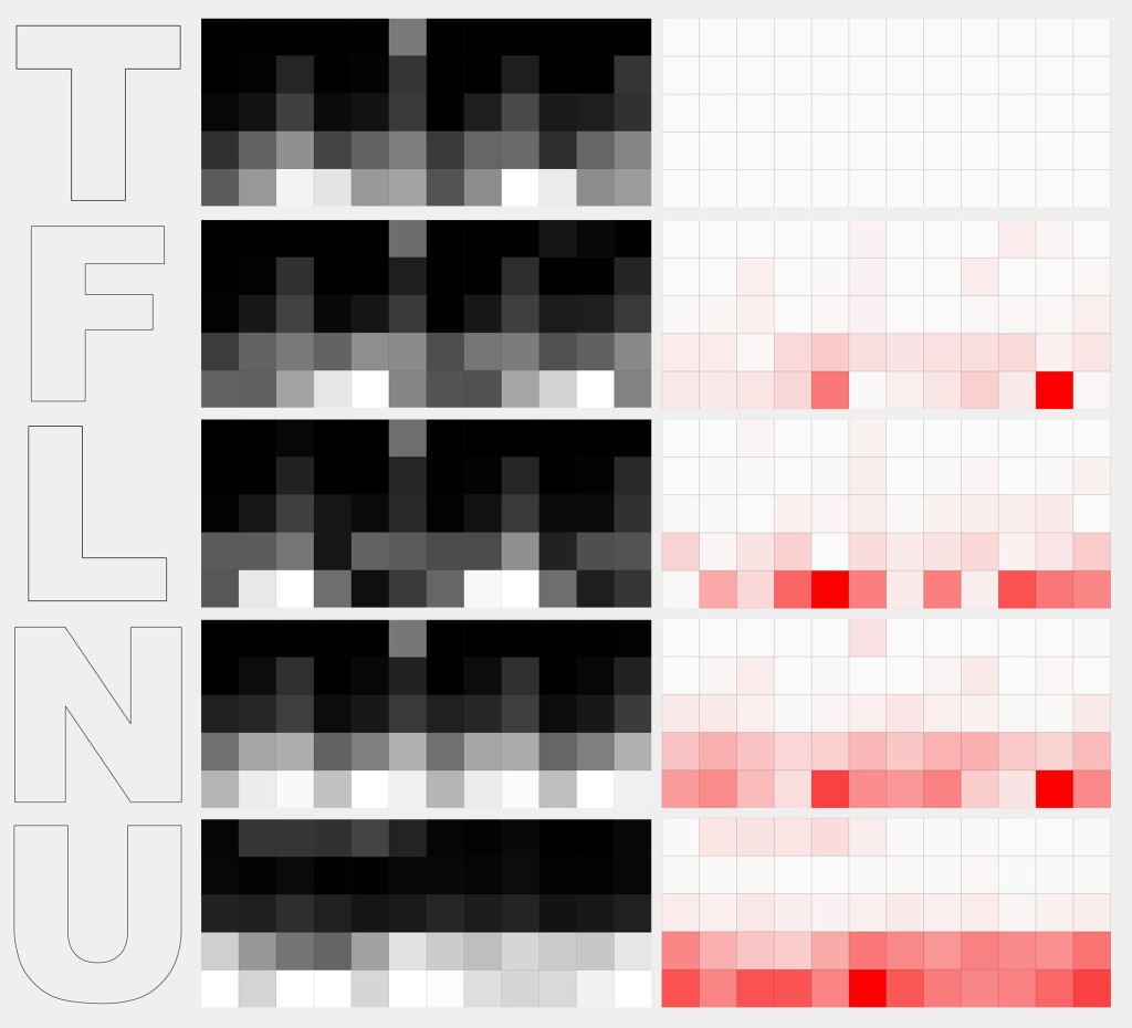
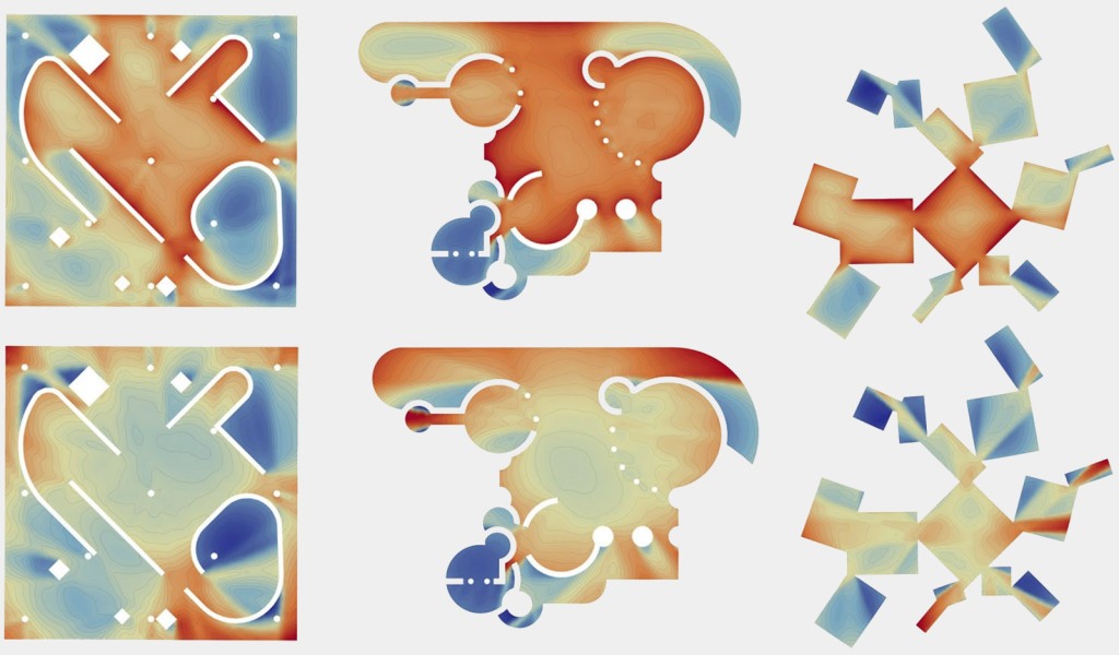
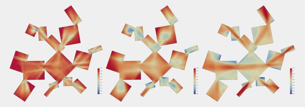
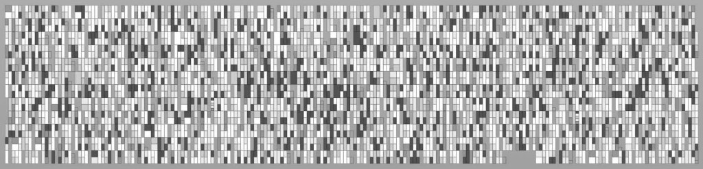
Similarity measure between different shapes. Left: Shape; Middle: “Global” shape context descriptor; Right: Difference between descriptors (reference shape is T). Similarity from top to bottom: 1.0, 0.834, 0.723, 0.796, 0.854

For some related reading:

S. Belongie, J. Malik, J. Puzicha: Shape Matching and Object Recognition Using Shape Contexts.

S. Belongie, G. Mori, J. Malik: Matching with Shape Contexts.

Transactions on Pattern Analysis and Machine Intelligence, vol. 24, no. 24, 2002

J. Nowak, R. Eng, T. Matz, M. Waack, S. Persson, A. Sampathkumar, Z. Nikoloski: A network-based framework for shape analysis enables accurate characterization of leaf epidermal cells. Nature Communications, 2021.

R. Veltkamp: Shape Matching: Similarity Measures and Algorithms

G. Franz, J. Wiener: From space syntax to space semantics: a behaviourally and perceptually oriented methodology for the efficient description of the geometry and topology of environments. Environment and Planning B: Planning and Design 2008, volume 35, p. 574-592.

N. Dalton: Synergy, Intelligibility and Revelation in Neighbourhood Places. PhD Thesis, 2010

SPHERICAL PANORAMA IMAGES

About two weeks ago, I wrote about visibility-based analysis and briefly mentioned spherical panoramas as a possible alternative representation to isovists and visibility graphs. This blog post goes into a bit more detail.

Isovists and visibility graphs are great methods to study the relationship between space and human perception and behavior. However, both methods do not account for visual properties such as color, texture, luminance, etc. which are important for human perception of spatial situations, as several studies have shown. This is especially true for the experience of spaciousness and openness, for which light and color are essential factors. For example, a room can appear larger if it receives more light, even though it is quantitatively smaller.

Such attributes like color, light and intensity are also often the visual features that are particularly eye-catching. The main tool for identifying the visual features that attract people’s attention is saliency. In the field of spatial syntax research, the effect of saliency has rarely been studied, and when it has, it has been mainly in relation to wayfinding and navigation. However, the use of spherical images to complement traditional visibility-based analysis methods allows for a more general approach in how saliency can be added to isovist analysis as a measure of human attention.

So how does this work? Well, technically it’s the same as rendering an image. But instead of producing a perspective image from a virtual camera, ray-casting is used to create a spherical 360-degree panorama image from any viewpoint specified by the user. In principle, it’s also very similar to the generation of isovists. The main difference, however, is how the ray directions are distributed and, in particular, how visible space is represented. Typically 360 degree images are either equirectangular or cube map projections. For simplicity, I use the former, which is a simple way to represent a sphere as a flat two-dimensional image by mapping plane coordinates to angles in polar coordinates around the viewpoint at its center. After casting rays in the directions of these angular coordinates, either various information is returned from the intersection point or further calculations are initiated. In either case, all derived information is stored in the corresponding pixel of an image. This might simply be, for example, the distance between the viewpoint and the first ray intersection point in the environment. But it could also be any number and type of data, such as the surface normal, surface luminance, color, etc., which are then stored in multiple layers in the image.

Utilizing spherical panoramic images for visibility-based analyses could open new possibilities and advantages, especially when combined with isovists and visibility graphs. Techniques from computer vision and image analysis, such as saliency detection, object recognition, image segmentation, etc., may enable an enriched notion of isovist measures and could greatly facilitate the exploration of spatial syntax in relation to human experience and perception. One such case, for example, could be the fact that being visible and being seen are not necessarily the same thing, as pointed out by Ervin and Steinitz. Saliency detection could be a way to consider and incorporate this fact in visibility-based analysis. Moreover, visualization and interpretation of three-dimensional isovists is no easy task due to the rather abstract representation and the large amount of data. Panorama images could be a step closer to solving this problem, since images are a very common way to represent space; people are used to understanding and interpreting them effortlessly. When using a VR player, for example, a panoramic image is a great way to give the user an interactive first-person experience of the environment by viewing it in the egocentric perspective from the given viewpoint. However, because people respond differently to features in a spatial context than they do when viewing images of scenes in a non-spatial context, such image-based methods are useful primarily to support isovist and visibility graph analysis but certainly not to fully replace it.

(The color artifacts are due to the GIF compression and not the result of the image generation)

And here’s a little example showing what it could be used for where I have basically done fellowing:

Generate a light/texture map
Cast rays into the scene and get uvs at the intersection point
Use the map to look up the color and luminance of the surrounding surfaces
Generate an equirectangular panorama image
Compute a saliency map for the image
Use the saliency map in a simple linear weighting function in the calculation of various isovist measures
Repeat the steps above for 100 uniformly distributed viewpoints

Instead of using it to weight different measures, we could also use the saliency map to weight the ray distribution for isovist generation, which would be similar to the concept of importance sampling in ray tracing. Applied to the context of visibility analysis, this would result in an attention-based ray distribution. In other words, we could use the saliency map to guide rays toward regions that are particularly eye-catching. And since ray casting is done on the GPU, the time required to shoot hundreds of millions of rays into the scene is negligible compared to the computation time for various isovist measures.

Equirectangular images are stretched horizontally at the top and bottom. These image regions correspond to the areas near the poles and are the result of mapping a sphere into a two-dimensional plane. Because of these distortions, saliency detection might fail and find visually salient regions in the image that do not exist at all in the “real” three-dimensional environment. To prevent this from happening, saliency detection was not applied directly to the rectangular panorama image. Instead, the image was processed in parts, similar to the method described in a paper by Startsev and Dorr. In my example it was done by extracting a perspective image with a horizontal view angle of 150 degrees and a vertical view angle of 135 degrees from the equirectangular panorama, which was then used as input for computing the saliency map. Once the map was created, it was converted back to the equirectangular format. This step was repeated for 30 iterations while the image region to be extracted was shifted horizontally by 12 degrees. The resulting overlapping saliency maps were stored in a multidimensional NumPy array and combined by taking the highest value along the third axis to get the final map corresponding to the original equirectangular panorama image.

TOPs FOR THE ARTS

This is a blog post I wrote about 3 years ago, but as it turned out today, I had never set it to public. Well, although now a few years too late (TOPs is not really new anymore), but here it is …

A good friend of mine is an artist who makes fantastic drawings, mainly with colored pencils. For many years he has refused to work with a computer, although it could be supplemental to his drawing process. However, the benefit of letting an algorithm do the heavy lifting every now and then is undeniable even for him. At some point he asked me to help him with one of his long-term projects for which he wanted to translate a large number of names into an abstract notation system he had developed years ago. Of course I said yes. Not only because I really like his artwork and we have worked together several times before, but also because it would be a perfect example for using TOPs. So, what he wanted to do was basically this:

Get a large number of names with seven letters (I still have no idea why it had to be seven letters …)
Generate all possible permutations for the names
Translate these resulting permutations into his abstract notation system

Translating a text into his notation system is something we already did a few years ago (I wrote about it in another blog post here). So this step was easy and didn’t take much work. Generating permutations for the names wasn’t much work either and was done by using Python’s itertools. The challenging task, however, was finding a good database of names from all around the world. Luckily there is the internet and after an evening of searching, we finally found a fairly large text file with a plethora of names. From that point on, it was pretty simple and straightforward to put together the setup in TOPs to generate around a thousand of such permutations . For the final large print, the permutations were rendered using an npr shader I wrote for the same friend a few years ago to give the pictures a somewhat hand-drawn look like here.

At each top left is the original name, at each bottom right the name in reverse order, and in between are all possible permutations.

VISIBILITY-BASED ANALYSIS

Well, it’s been a long time since my last blog post. Free-time is rare and (un)fortunately there is a rather long list of unfinished projects I could and probably should continue working on. One of these projects and a topic that has generally interested me a lot for many years is the large field of visibility-based analysis. A few years ago I wrote a short blog-post about it here. Since I’ve been working on it again in the last few months and have rewritten most of the old implementation, I thought it might be a good time for an update.

On a conceptual level, visibility-based analysis methods are quite fascinating, as the relationship between visuospatial properties and psychological responses and behavior is one of the most important considerations in how people interact with and in their (built) environment. On the computational and algorithmic level, it is quite a challenge to make it accurate, fast, and memory efficient at the same time, especially for a three-dimensional environment. This starts with the generation of an accurate representation of visible space (in other words, a two- or three-dimensional polygon/polyhedron) and ends with the computation of various geometric and topological measures based on those structures. The general principle of spatial analysis is not hard to understand, but getting deeper into the concepts does take some time. This is especially true for the various quantitative measures and their meaning. A great deal of research has been done in the last forty years, a considerable amount of which has come from the fields of psychology and philosophy.

Visibility-based spatial analysis is a way to investigate and understand the relationships between (visible) spatial properties, (human) experience, emotional associations, and behavior. From a conceptual and computational perspective, there are currently two main approaches. The first approach is called isovist analysis and is mainly concerned with geometry, the second is based on the mutual visibility of points and is summarized under the term visibility graph analysis (VGA). While isovists deploy geometric-spatial information for a particular position in space, VGA unfolds the topological relationship of different positions in space to each other.

In order to explore space to its full extent, it is imperative to complement the typical two-dimensional analysis with a three-dimensional method. For that reason, three different approaches have been implemented: a (1) geometry-based, a (2) topology-based, and an (3) image-based method (which will be the topic of another blog post …).

At its core, any visibility analysis application has to meet several requirements: (1) fast ray-casting for (inter)visibility computation, (2) geometry and/or graph generation, (3) data analysis and manipulation, and finally (4) data visualization. Since Houdini is more than capable in all these areas, it was the logical choice for the software framework on which I developed and implemented such a tool. Many of the algorithms have been written either in VEX or, to take advantage of today’s GPU processing power, in OpenCL. To keep the entire toolset as flexible and accessible as possible, only a few algorithms are written in C++ using the HDK. All in all, it’s about 67.500 lines of custom code and 1683 nodes.

Without going into detail, here are some basic examples of what it can do:

Generate axial lines (all axial lines and fewest axial lines)
Generate spatial partitions (s-partition and e-partition)
Compute a sufficient set of points and isovists (based on a fast iterative algorithm to approximate the famous art gallery problem)
Generate movement patterns (based on various spatial measures)
Two- and three-dimensional isovist an visibility graph generation
360° spherical panorama image generation to supplement three-dimensional isovist analysis

Top left: all axial lines and fewest axial lines; Top middle: s- and p-partition; Top right: sufficient set of points and isovist polygons; Bottom left: movement pattern; Bottom middle: 2D/3D isovist (bottom: tri-planar and contour 2.5 D isovist); Bottom right: 360° spherical panorama images (lighting, depth)

Isovist Generation

For the generation of two- and three-dimensional isovists, I’m using two different methods. (1) One method is based on simply sending rays from the “viewpoint” radially into the scene. This works quite robustly (no problems with overlapping and/or intersecting polygons) and is very fast, since ray casting is implemented to work on the gpu. However, the resulting isovist is always an approximation but not an accurate representation of visible space. This becomes even more apparent for areas farther away. Because rays are distributed evenly over a circle/sphere around the viewpoint, distant areas of the environment are captured in less and less detail. (2) The second method circumvents this problem by computing an accurate isovist. To do this, a sweep-line algorithm is used which relies on the connectivity structure of the mesh. The resulting polygon/polyhedron consists of vertices and edges only at the exact intersections with the 3D environment and is therefore an exact two/three-dimensional representation of visible space around a particular viewpoint. In the image below, you can see the area difference between exact isovists (sweep-line algorithm) and isovists created by simply radially sampling the scene (radial ray-casting algorithm).

Left: radial ray casting – 180 rays, area difference of max. 29.6 m²; Middle: radial ray casting – 360 rays, area difference of max. 12.6 m²; Right: radial ray casting – 720 rays, area difference of max. 7.3 m² (Well, instead of using absolute values, I should have expressed the difference in percentages, so that it actually would make sense …)

Top left: isovist based on radial ray casting; Top right: isovist based on radial sweep line algorithm; Bottom left: 360° isovist (left: radial ray casting, right: radial sweep line); Bottom right: partial isovist.

Three-dimensional isovists are generated in basically the same way as two-dimensional isovists, again as an approximation (radially casting rays) or by calculating geometry intersections for an accurate isovist representation of visible space.

Visibility Graph Generation

Conceptually and computationally, there is no difference between a two-dimensional and a three-dimensional visibility graph. In any case, it’s based on the mutual visibility of points. Thus, the whole space is usually divided into smaller same-sized parts. In other words, the sample points are evenly distributed in a grid-like structure over the entire domain (surface/volume). However, we can also specify a second set of points. Thus, it’s possible to use a very dense, high-resolution pointset as “viewpoints”, but to use considerably less points as “target points” for checking indivisibilities and constructing the graph. To get meaningful results for the analysis, the varying density is then compensated by a multiplication factor based on the spatial area/volume around each sample point.

Top left: accurate isovist; Top middle: approximated isovist; Top right: visible points (voxels) from a particular viewpoint; Amount of visible space (volume) visualized as points (bottom left) and as isosurfaces (bottom middle); Bottom right: Amount of visible space (volume) from sample points (viewpoints) at 1.7 m above floor level.

Measurements

Currently, about 100 different local and global isovist and visibility graph measures can be calculated. These include many well know measures as proposed by various authors in the space syntax literature, such as area, circularity, drift, clustering coefficient, visual integration, etc., as well as less common measures such as revelation, angular correlation, fractal dimension, local symmetry, and so on. Each can be based on first and/or second order visibility relations and most work in both, two- and three-dimensional domains. In addition to already existing spatial descriptors, several new ones have been implemented. Some of them are shown below.

Similarity: Based on the visible neighbourhood of 0.5 m (left), 2.0 m (center) and the entire visible neighbourhood (right) per sample point.

Boundary Similarity: Based on solid and occluding edges. Similarty between continuous (middle) and single edges (right).

Local Symmetry: Degree of experienced symmetry from the ego-centric view (left). Sreamlines along the local (middle) and semi-global (right) symmetry vector.

Predictability: Based on the visible neighbourhood of 2.0 m (left) and the entire visible neighbourhood (right) per sample point.

Deflection: Local (left) and global (right) deflection

Conceptual and Methodological Framework

Although isovists and visibility graphs are both used for spatial analysis, they are fundamentally different from a conceptual and mathematical point of view, as mentioned earlier. Summarized the main differences are (isovist left, visibility graph right):

Geometric representation of space
Represents the shape of space
Observer-centric and therefore (typically) local description of space
Conceptually a continuous approach
There is a strong relationship between the isovist geometry and psychological and emotional response

Topological representation of space
Represents the space in terms of spatial relations
Typically global description of space
Conceptually a discrete approach
Conceptually, there are similarities to models of spatial memory from cognitive science

On a conceptual level, the general implementation largely follows Sophia Psarra and Sam McElhinney’s proposal to discard the distinction between isovists and visibility graphs, and instead reinterpret a combination of both concepts as a “relational framework” of geometric entities. In this context, the term “relational” refers not so much to the mutual visibility of points in the graph, but rather to how isovists relate to each other in terms of overlapping areas. To prioritize a purely geometric approach as much as possible, overlapping regions are therefore described by “sub-isovists” rather than by topological information based on the intervisibility of points. Conceptually, this method pursues a continuous approach and is thus independent from the number and distribution of sample points. Topology-based computations are thus largely replaced, not least to stay consistent with the conceptual and theoretical basis on which the implementation is built. Apart from this, it is quite satisfying to watch the isovists and subisovists changing continuously when moving from one position to another (animation below).

Sub-isovist generation

First and second order visibility relations between points and isovists.

Of course, this is not the only tool for visibility-based spatial analysis. The best known applications are most probably depthmapX by Tasos Varoudis and the Isovist app by Sam McElhinney. Both applications have been very helpful for comparing and cross-checking many analyses results. So, big thanks to Tasos and Sam for making both tools freely available. Following their example, I will make my tool available as well, as soon as I’ve cleaned up the coding-mess a bit.

Although all these methods originate mainly from architecture and urban planning research, they are also quite interesting for space planning in the generation of game environments. For example, they could be used to generate and/or optimize a spatial structure in terms of its spatial intelligibility from the egocentric perspective of a player. Take, for example, a maze. It could be generated to be highly differentiated and surprising at the local level (visible space from a particular point), but clearly structured and memorable at the global level (the overall structur of it). Or it could be the opposite.

For some related reading:

Turner A, Penn A (1999) Making isovists syntactic: Isovist integration analysis: Proceedings of the 2nd International Symposium on Space Syntax, vol. 3

Turner A (2001) Depthmap: A program to perform visibility graph analysis: 3rd International Symposium on Space Syntax, Georgia Institute of Technology

Benedikt ML (1979) To Take Hold of Space: Isovists and Isovist Fields. Environment and Planning B 6:47–65

S. Psarra, S. McElhinney (2014) Just around the corner from where you are: Probabilistic isovist fields, inference and embodied projection. The Journal of Space Syntax, vol 5

G. Franz, H.A. Mallot, J.M. Wiener (2005) Graph-based models of space in architecture and cognitive science – A comparative analysis

D. R. Montello (2007) THE CONTRIBUTION OF SPACE SYNTAX TO A COMPREHENSIVE THEORY OF ENVIRONMENTAL PSYCHOLOGY

Dalton N Synergy, inteligibility and revelation in neighbourhood places. Doctoral thesis, UCL (University College London)

Krukar J, Manivannan C, Bhatt M et al. (2021) Embodied 3D isovists: A method to model the visual perception of space. Environment and Planning B: Urban Analytics and City Science 48:2307–2325

Bhatia S, Chalup SK, Ostwald MJ (2013) Wayfinding: a method for the empirical evaluation of structural saliency using 3D Isovists. Architectural Science Review 56:220–231

FROM NORMAL MAP TO HEIGHT MAP

The question is why do we want to have height maps instead of normal maps in the first place? Well, there are various reasons but the most obvious are that they are easier to edit, generally easier to understand and the result, when applied as displacement map, is easier to anticipate. In other words, while normals maps do have some advantages, they are generally less intuitive to work with and that’s probably a good reason why we might want to convert them. But before going into details how the conversion is done, let’s quickly recap what a normal map is and how it could be generated.

In fact it’s pretty easy and hence we’ll set up a simple example. Let’s take a grid, for example, and apply a noise function to it (in our case a mountainSop). Next compute point normals for the deformed grid and encode these normals as colors. Finally just write out the colors as texture map or directly generate the map by using the texture baker. And basically that’s it, the result is our normal map.

But now let’s reverse the process and assume we have our normal map but the geometry is just a flat grid. How can we reconstruct the original deformed geometry?

Well, let’s start simple. As we already know and the name “normal map” implies, normals are encoded as colors. To be more precise, the rgb values of our map correspond to the xyz components of the normals we are searching for. This means we can pretty much do a 1:1 conversion. The only thing we have to take care of is changing the range from 0, 1 (colors) to -1, 1 (normals). If we’ve done that we indeed end up with proper normals, the grid however, is still flat. What we need to do next is adjusting the points position/height so that the displaced grid finally matches the original deformed geometry. And that’s the tricky part. So, the question now is how are we going to get the height information out of our normals?

Well, one way for instance, is trying to solve this problem geometrically. This could be done by iteratively moving the points vertically up/down until new computed normals match the ones we got from our normal map. For a simple mesh/map this technique is fast and reasonably accurate but for more complicated maps and/or irregular meshes it starts failing and the result might just not be what we’d have expected. To overcome this problem there exist various other methods which could be used instead but my personal favourite is, once again, to rely on the famous Poisson equation.

If we assume height is a function on the mesh, it can be computed by minimizing the difference between our pre-computed normals (projected onto the tangent plane on the mesh) and the gradient of this function in the least squares sense. Since this is leading to the Poisson equation it’s easy to set up a linear system in the typical form A x = b. If we then use a fast sparse matrix library and let it do it’s magic by solving the system for x, we finally get what we were looking for, namely our desired height.

And of course, it works on non-flat meshes too.

Instead of setting up and solving everything in matrix form it’s also possible to do it with VEX/OpenCl although the setup is a bit different and it takes longer to solve. Anyways, for those who don’t have access to a fast matrix solver it’s a reasonable alternative. The process is pretty much the same as it’s done in this blog post.

THE JOY OF USING MATRICES

Fom VEX/OpenCl to sparse matrices

In my last blog post I wrote a bit about the possibility to (mostly) circumvent the need of using sparse matrices in Houdini and instead setting up and solving the system in VEX/OpenCl. This time, however, it’s about the other way around and how a typically VEX/OpenCl based setup could be implemented and solved in matrix form.

Pretty much everybody using Houdini has at some point done basic Laplacian smoothing on a mesh (with uniform weights), perhaps without even knowing it. It’s a widely used algorithm and fairly easy to implement by averaging the values of the 1-ring around the current point. In fact, in Houdini it’s even easier than that and we can just use the attribBlurSop. AttribBlur is using OpenCl under the hood and relies on the basic graph Laplacian to blur/smooth point data, such as P for instance. This is done by performing the smoothing/averaging step a number of times which is conveniently exposed as iteration slider in the UI of the attribBlurSop.

However, this is of course not the only way how Laplacian smoothing could be implemented. Instead of iteratively applying the smoothing step per point we could also set up a simple linear system and solve it subsequently for the final point positions. This is what I’ve done in the file below. It’s a simple example where I’m using a direct solver in Scipy which is basically solving all the equations simultaneously in one go.

In practice it doesn’t make much of a difference which method we use because both will lead to the same result in pretty much the same amount of time (at least for our example). But since Laplacian smoothing is already provided to us by the attribBlurSop it’s most probably best to just use what’s already there instead of implementing it in matrix form.

Anyways, apart from practicality I hope this simple example, together with my last post, helps to clear up some misunderstandings and the question if it’s absolutely necessary to use sparse matrix libraries in Houdini or not.

FILE

ps.: To run the example file without problems you’ll need to have Scipy installed on your system/computer.

THE JOY OF NOT USING MATRICES

From sparse matrices to VEX/OpenCl

Over the last months I had some conversations about the need of using (sparse) matrices and/or matrix solvers in Houdini to implement various fundamental algorithms for geometry processing, such as the Poisson Equation. Of course, most of the time we definitely want to work with matrices because everything is easier to understand, faster to set up, and also faster to solve. Nevertheless, I think it’s important to know, that even if that’s the prefered method, it’s not the only one. This becomes particularly apparent when working with Houdini because it doesn’t get shipped with Scipy or any other easy-to-use sparse matrix library. So, as long as we don’t want to compile Scipy by our own, we’re stuck with either using Numpy (which doesn’t support sparse matrices) or using the HDK.

However, the good thing is that if we don’t want to, we do not have to use matrices at all. In other words, if we don’t have access to Scipy and don’t want to use the HDK, pretty much all of it can also be done in VEX and/or OpenCl. It will be slower and most probably less accurate but it works by only using standard SOPs without the need of external dependencies such as Scipy, EIGEN, …

About two years ago I wrote a little blog post about various algorithms how to compute geodesic distance fields on meshes. Nowadays we can simply use surfacedist() but back in 2017 you had to code it by yourself. And of course, if someone is talking about geodesics, there is no way of getting around Keenan Cranes wunderful paper “The Heat Method for Distance Computation”. So, what would be a better example than an implementation of exactly this paper!?

I won’t go into details about the method described in the paper since everybody should read it but it works by basically solving the heat, as well as the Poisson equation. Both are typically set up and solved as a linear system in matrix form and that’s also what I did for my “Geodesics on Meshes” Blog entry. This time, however, we are going to do it differently and use only standard SOPs together with a bit of VEX and OpenCl.

Gradient
Geodesic distance field
Heat integration

So, below is the file with two slightly different methods. Example one is simply using Jacobi iteration to solve the heat and Poisson equation and example two is relying on Successive Over-Relaxation to speed up convergence time (if Jacobi takes n iterations, SOR convergence in approx. sqrt(n) iterations depending on the relaxation factor). Additionally for reference and/or performance comparison there’s also an example which uses sparse matrices in EIGEN together with the HDK and another one which uses Scipy. To run the HDK example you’ll need a working compiler since it’s implemented by using inlinecpp() and for the Scipy example, well, you’ll need Scipy.

FILE

K. Crane, C. Weischedel, M. Wardetzky: The Heat Method for Distance Computation

MESH DEVELOPABILITY

Some weeks ago I had an interesting conversation on the Houdini Discord Server about Keenan Cranes fairly new paper Developability of Triangle Meshes. The paper is, of course, excellent as always and the topic quite interesting in general. Nevertheless I somehow missed it when it was officially published and even worse – I completely forgot about it although I was at a conference around two years ago where Keenan Crane gave a beautiful talk about their new method. Fortunately there are people around who are really quick in finding new papers and after it was pointed out to me by Spinynormal I did a quick and dirty implementation in Houdini. It’s just a rather rough prototype without taking too much care about all the details but nonetheless it seems to work quite well.

To be honest, at the time when I saw Keenan Cranes talk I was first a bit sceptical. I really liked the idea and thought wow, that’s brilliant but I also had my doubts about the practicality of their method. Since the result depends largely on the structure of the mesh and not so much on it’s shape (or other properties), flipping some edges, for instance, might lead to a very different solution. And to put it simple, it wasn’t sure if this is an advantage or rather the opposite. Well, now, years later and after playing around a bit with the implementation in Houdini, I’m pretty much convinced that it’s an advantage. It’s quite interesting to watch how the mesh evolves into different shapes by just changing small parts of the triangulation. But then again, I don’t need to use it in practise.

K. Crane, O. Stein, E. Grinspun: Developability of Triangle Meshes

FIELD GUIDED REACTION DIFFUSION

Just some fun doing direction field guided reaction diffusion with OpenCl.

POLYGON PLANARIZATION

Last week I had a great conversation with someone in the Houdini discord chat group about an interesting problem. He had a surface made up of quads and wanted to “planarize” the polygons in order to build a large physical model from it. He told me that he usually uses Grasshopper and Kangaroo for this but was wondering if it’s also doable in Houdini. Well, I don’t know Kangaroo very well but as far as I know it’s basically a particle-spring based solver. It uses a force based approach which works quite well for many different problems such as planarizing a polygonal mesh. (This isn’t true any more! Daniel wrote me in the comments below that Kangaroo is using a projective solver since 2014). Pretty much the same, of course, could be done in Houdini. By using a “planarization force” together with constraints in the grainSolver it’s easy to replicate such a system. Instead of using grains it’s also possible with wires. Most probably they’re not as stable as grains but nevertheless it should do the job. If we like we could also build our own force based solver. Implementing verlet integration in a solverSop is easy and apart from that there’s the gasIntegrator microsolver which we can use in DOPs for that purpose. However, to get a stable system it’s important to choose the right step size for the integration. If it’s too large the system explodes and if it’s to small it takes forever to find its equilibrium. Of course, higher order integrators like Runge Kutta are minimizing this problem and generally they are quite stable. The same is true for the position based approach of grains but the problem still remains, at least to some degree.
Anyway, it’s an interesting problem and even though it’s typically not too hard to solve it could become quite tricky depending on the geometry. The hard part is not so much to obtain planar polygons but to stay as close as possible to the original mesh. In the worst case we might end up with an entirely flat mesh what’s clearly not the intended result. The reason might be, for example, that the mesh describing the surface has an unfavourable structure. And sometimes it’s simply not possible because not every surface can be made up of planar polygons except triangles.
During our chat I remembered that there was a thread on OdForce about pretty much the same topic. Someone had a saddle-shaped surface for which he computed the dual mesh and subsequently wanted to make the resulting hexagons planar. At the same time the boundary points of the surface should keep their original position. Well, even though a saddle surface seems to be rather simple, it is not and I think this is a good example to highlight some of the problems we might run into when we’re trying to planarize polygons.

But first let’s take one step back and start simple. Instead of using hexagons let’s assume it is a quad mesh. One way to tackle this problem is to use a force based approach similar to what Kangaroo/Grasshopper is doing. We need to set up a number of forces and run the system until it reaches equilibrium. To calculate the “planarization-force” we could, for instance, project the polygon points onto the plane defined by center and normal. Or we compute the diagonals and check their distance to each other. To preserve the mesh structure we can rely on edges and diagonals as spring forces. Additionally we need to keep the points of the boundary at their position. The key point, however, is to adjust the weighting between all these forces to finally get the result we were looking for. Usually there is no way to find a solution satisfying all the objectives and hence the result is highly depending on how we balance the forces. As said above, such an approach is easy to set up and it works quite well under most circumstances. However, for a number of reasons I thought it might be better to take a slightly different approach. Instead of using a force based system I used a method which is conceptually somewhat similar to the “As Rigid As Possible Surface Modelling” approach. Intuitively it’s easy to understand and works basically in the following way:

For every polygon of the mesh, the planar counterpart is computed and then fitted to the original poly in the least squares sense. For our specific “planarization problem” we could also just project the points onto the tangent plane but in general we may want to rely on rigid shape matching to find the best fitting orientation. This could be done easily in VEX by using polardecomp() or by using Numpy. Even though polar decomposition in VEX is faster I tend to use Numpy’s SVD algorithm since it doesn’t have problems with flat axis aligned polys. Of course, we could make our matrix positive by adding a very small value but this might lead to other problems instead. For a high number of polygons it’s a good idea to implement a simplified SVD algorithm in VEX which doesn’t have such problems but in most cases Numpy should be fast enough. But let’s not get off the track and back to the planarization problem.
After the “planarization” step is applied to each polygon the mesh is obviously torn apart. What we need to do next is to reconstruct the mesh in the least squares sense based on the planar polygons. In other words, we need to set up and solve a linear system. If we repeat these steps iteratively a number of times the system finally converges to the solution we are looking for. The result is the mesh made up of planar polygons. So, the process boiles down to the following threes steps:

Fit planar polygon to original polygon in the least squares sense
Reconstruct mesh based on planar polygons in the least squares sense
Repeat until system converges

Of course, we also need to implement all the other constraints too, such as fixed boundary points, mesh structure preservation and so on. In the example below, the four corner points are fixed at their position all the other points are allowed to move in all directions. In my tests the algorithms works quite well and is also relatively fast. For the mesh shown below it needs about 175 iterations and converges in about 280 ms on my rather old laptop.

But now let’s go back to the example file from OdForce. The original question was how to obtain planar hexagons while retaining the overall shape of the mesh. Additionally, even though it’s not mentioned in the post, we may want to keep the mesh structure intact. In other words, the polygons should stay connected. Well, this sounds easier than it is. It is indeed possible but we might end up with unwanted results. The problem is that the saddle-shaped surface has negative gaussian curvature and hence it can’t be approximated by convex hexagonal polygons. However, if we allow non-convex polygons it’s doable although the deviation to the original shape is rather large. This is clearly visible in image 2 and 3 below. If we additionally allow for open edges the overall shape is preserved very well (image 4). However, this is just the case for hexagonal polygons and won’t work for quads in the same way. So let’s take a look what happens if we choose four-sided instead of six-sided polygons.
(Side note: For computing planar hexagonal meshes it’s most probably more efficient to rebuild the mesh instead of planarizing it’s polygons but that’s maybe a topic for another blog post)

Planar non-convex polygons with open edges

Planar non-convex polygons with connected edges

Using the planarization algorithm on the quad mesh results in a completely flat surface which is clearly not what we want. But how could this happen? Well, the simple reason is that it’s just not possible to obtain planar AND connected polygons based on our initial mesh without getting large deviations in the overall shape. This is clearly visible in the images below. Picture 1 is the original mesh made up of non-planar polygons. Picture 2 shows the result of the planarization with fixed corner points and picture 3 is the planarized poly mesh without any additional constraints.

Planarized mesh with fixed corner points

So what can we do to get a better result? The answer is simple. We need to provide a better starting point for the algorithm. In other words, we need to remesh the surface. The most natural way to remesh a surface is based on it’s principal curvature direction. By integrating the fields, for example, we could extract a conjugate curve network which we then use to construct the mesh. Such a curvature aligned mesh is exactly what we need since it’s quads are naturally close to planar. For simple geometries this is not too hard to implement and the resulting mesh is a perfect starting point for the subsequent planarization algorithm. In the case of our saddle-shaped surface it’s even better because we don’t need to do any planarization at all. The new curvature aligned mesh is already composed of fully planar polygons.

For some related reading:
R. Poranne, E. Ovreiu, C. Gotsman: Interactive Planarization and Optimization of 3D Meshes
S. Bouaziz, S. Martin, T. Liu, L. Kavan, M.Pauly: Projective Dynamics: Fusing Constraint Projections for Fast Simulations
W. Wang, Y. Liu: A Note on Planar Hexagonal Meshes
W. Wang, Y. Liu, B Chan, R. Ling, F. Sun: Hexagonal Meshes with Planar Faces

CURVES … appendix

My last blog post was mainly about curves and how some of the tools known from Grasshopper/Rhino could be implemented in Houdini. Somewhere at the very end of the entry I mentioned inflection points but I didn’t explain what it is. Well, I’ll try to do it now.
An inflection point is a point on a curve at which the curvature changes sign. For example, when we look at a two dimensional s-shaped curve and visualize it’s normals then there’s a point at which the normals flip from one side of the curve to the other. This point is the inflection point. Not every curve does have such a point but if it has one (or several), it’s sometimes useful if we know how to find it. For instance, it was important in the example in which I was approximating a curve by circular arcs. However, the inflection point is just an example and maybe we need to search for other points, such as global or local extreme points, points of max. or min. curvature and so on.
To find such a point we basically have two options. One way is to recursively sample the curve in smaller and smaller steps until we get the point of our interest. This is easy to implement and works generally very well for all kinds of curves. A more elegant and more accurate method, however, is to remember that we are dealing with polynomials and hence to find the point analytically. In case of searching for the inflection point this simply means that we have to solve the polynomial for the point at which curvature is zero.

CURVES

From time to time I’m having interesting talks with people who are mainly using Grasshopper and Rhino for their job. They are working in the field of architecture and/or design and even though they are usually quite interested in Houdini one of the first things I always hear is how bad the curve tools are compared to Rhino/Grasshopper. Well, that’s not true! Or let’s say, it’s just half the truth. Even though curves, and Nurbs in general, could get some love they are quite robust and not too bad to work with. (As long as we don’t need to fiddle around with trimmed surfaces). Houdini is not a CAD program and naturally it doesn’t have all the features which are available in Rhino/Grasshopper. So, when I asked what the main curve tools are that Grashopper users are missing the most in Houdini I got a list with the following five points:

Curvature
Curvature graph
Curve deviation
Curvature based resampling
Approximate curves by circular arcs

Of course, there are many other things which are missing, for instance, better handles to create and modify curves but since the points above seem to be the most important features to Grasshopper users I’ll stick with those. However, curves are not too complicated and if you ever need to implement or generate “custom” curves there’s plenty of good information available online. For a start you could take a look at these simple example files on OdForce.
But now back to the missing feature list. Before we start, it’s important to note that there are mainly two different kinds of curves in Houdini. On one hand we have Nurbs and Bezier curves which are basically polynomial curves parameterized by a function. On the other hand we have polygonal curves which are usually just points connected by straight lines. If we like, we could call the two types smooth and discrete curves.

Curvature
Curvature is fairly easy to calculate if we understand what it actually means in the context of curves. Basically it tells us how fast a curve is changing direction when we travel along it. In more mathematical terms, it’s the magnitude of acceleration. So far so good but what exactly does this mean? Well, acceleration is the second derivative, or in other words, the normal of the curve. The first derivative is velocity or slope and this is nothing more than just the tangent. So, if we want to compute curvature it comes down to implementing the following three simple steps:

Compute first derivative namely the tangent
Compute second derivative (which is the normal) based on tangents
Measure magnitude of normal which finally is curvature

A nice side effect of this procedure is that we can easily compute a local frame since we already have tangent and normal. We just need to compute the cross product of these two known vectors and we’ll get the third vector and hence an orthogonal local frame on our curve. To get the osculating circle at a given point, like it’s possible in Grasshopper, we need to calculate the radius which is just the inverse of curvature.
All this is relatively easy to implement in VEX, both for Nurbs and polygonal curves and it’s also quite fast. However, for discrete curves the easiest method is most probably the use of a slopeChop in CHOPS. On OdForce there is a rather old example file using this technique to compute the Frenet frame. It’s not exactly about curvature but it shows the general setup.

Curvature graph
Well, this is easy because it’s just the normals reversed and scaled by curvature and a multiplier by the user.

Curve deviation
This is easy too. We just need to use xyzdist() at sampling points on the first curve to get the distance to the second curve.

Curvature based resampling
This is again a job for xyzdist() which we could use to implement our own curve sampling algorithm in VEX. This could be done based on a minimal distance or maximal angle threshold by using a bit of basic trigonometry together with the xyzdist() and primuv() combo.

Approximate curves by circular arcs
This was the most important point on the list what makes totally sense for applications in the field of architecture and design. If someone is actually going to built something physically it might be a good idea to find a way how to approximate an arbitrary 3D curve by circular arcs as close as possible. So, how could we implement this in Houdini? Well, there are many different ways but the easiest would be to “brute-force” it. Since an arc is well defined by three points we could start with two close points at one end of the curve. Next we find the point in between construct an arc and estimate the maximal deviation to the curve. If it’s smaller than an user given threshold increase the distance between the points and repeat the steps until we get the largest arc within our tolerances. Then we just repeat the whole procedure until we finally get our arc approximated curve. VEX is pretty fast and hence this algorithm should work quite well performance-wise, even for very dense resampled curves.
However, I thought it might be better to choose a different and probably smarter method. The reason is mainly because the approximation should be as smooth as possible without large kinks along the curve. Instead of using the algorithm described above, which is not guaranteed to result in tangent arcs, we could use a method called biarc fitting. So, what is a biarc? A biarc is a pair of two arcs with the same tangent at the point at which they meet. And this is exactly what we need for a good and smooth approximation of the curve. The general algorithm is fairly easy to implement and works basically as follows:

Get tangent at endpoints
Sample curve and search for best connection point for biarc
Estimate deviation between biarc and curve
If deviation is larger than given tolerance split curve and repeat
If deviation is smaller than given tolerance compute the biarc

Instead of using just the distance between biarc and curve I’m using various different measurands to estimate the error, such as max. distance, average distance, torsion angle and tangent angle. The images below show some results using the distance with different tolerance settings. Of course, there are some things we need to take care of, for instance, splitting curves at inflection points but generally biarc fitting is fairly easy to implement and works quite well for all sorts of curves.

Nurbs curve

Circular arc approximation

FIEDLER VECTOR AND THE CURVE SKELETON

Computing curve skeletons of 3D shapes is an important tool in computer graphics with many different applications for shape analysis, shape matching, character skeleton construction, rigging and many more. It’s an active field of research and over the years, numerous algorithms have been developed. Most of these algorithms are based on mesh contraction using smoothing or thinning. Another popular approach is to use the voronoi diagram generated by the points of the mesh. Quite an interesting alternative, however, is to rely on spectral analysis for computing the skeleton. The idea is fairly simple and works as follows:

Compute the first non-zero eigenvector of the Laplace-Beltrami operator, namely the Fiedler vector.
Compute contour lines based on the Fiedler vector
Find the center point for every contour
Fit curves to the points

VECTOR FIELDS … AGAIN

I guess I know what you think: “Not again another post about vector fields!” Well, that might be true but vector fields are omnipresent in computer graphics and therefore it’s incredible important to get a basic understanding of vector calculus and how it’s used in Houdini. A vector field is, as the name implies, a field of vectors in n-dimensional space. In Houdini terms, it’s a bunch of vectors assigned to points, vertices, polys or voxels of a mesh or a volume. That’s roughly what a vector field is. It’s easy to understand and easy to visualize. However, much more interesting than what it is, is to know what we can do with it and how we compute it. And that’s exactly what I’m trying to explain in this blog post. I’m not going into all the details but trying to give a general overview in the context of Houdini’s Surface Operators, better known as SOPs.
So, how do we compute a vector field in Houdini? Well, honestly, there is no single answer to this question because it mainly depends on what kind of field we would like to generate. One of the most important vector fields, however, is the gradient vector field. So, what is a gradient vector field? The gradient is the first order derivative of a multivariate function and apart from divergence and curl one of the main differential operators used in vector calculus. In three-dimensional space we typically get it by computing the partial derivatives in x, y and z of a scalar function. In other words, if we apply the gradient operator on a scalar field we get a vector field. Well, that’s more or less the general definition but what does this mean in the context of Houdini? I’ll try to explain it on a simple example.

Lets create a grid, wire it into a mountainSop and we’ll get some kind of a landscape like in the images below. Now let’s have a look at different points on that “landscape” and measure their height. For every of these positions, the gradient is the direction in which the height (P.y) is changing the most. In other words, it is the direction of the steepest ascent. We could check this by simply sampling the height values of our landscape around the points. Just copy small circles onto the points, use a raySop to import the height attribute and search for the point with the largest value. This way we get a good approximation to the gradient, depending on the number of sampling points. Of course, that’s not how the gradient is computed but it might help to get a better understanding of it’s meaning. The height is simply the scalar input for the gradient operator and the result is a vector. If we apply the gradient operator on every point of the geometry, we finally get our gradient vector field over the mesh.

Vector pointing into direction of steepest ascent

So far so good, but what’s so special about the gradient vector field you might ask. Well, a gradient field has several special and important properties and we are going to explore some of them by having a closer look at our previous example. For instance, if we generate contour lines of the scalar field (our height attribute which is the input for the gradient operator) we can see that the vectors are locally perpendicular to the isolines. If we rotate the vectors by 90 degrees, or rather compute the cross product with N, we get a vector field which is tangent to the contour lines. While both vector fields are tangent to the surface, the rotated vector field is in terms of its properties pretty much the opposite of the gradient. I won’t write much about it since I already did in another post, but nevertheless it’s important to mention what the main difference is. The gradient vector field is curl-free, it’s rotated counterpart, however, is a solenoidal vector field and hence divergence-free. If the field is curl- and divergence-free, it’s a laplacian (harmonic) vector field. But let’s go back to the gradient for now and have again a look at our “landscape” example.

Imagine, you’re standing on the top of the hill, put a ball on the ground and give it a light push in a specific direction. Most probably the ball will start rolling and if you’re not fast enough to stop it, it’s rolling down the hillside to the very bottom of the valley. Well, that’s nothing special and not much of a surprise. What is special, however, is the path the ball will take on its way down. It’s the path on which the height decreases locally as fast as possible and this route is exactly following the gradient vector field, or more precisely, the opposite direction in our example. This principle is called gradient descent/ascent and is used extensively for local minimization and maximization problems, as well as for local optimization problems in general. But mind, the keyword here is local. For global optimization problems we have to use different methods. This is quite obvious if we again look at our example. Depending on the sample point, or rather starting point of our path, we reach the local but not necessarily the global minimum/maximum. To make sure, that we actually find the global minimum, in other words, the point at the very bottom of the valley, we have to use a rather large number of samples.
Since the paths are following the gradient vector field, they are perpendicular to the contour lines of our height field and together they form a network of conjugate curves. Conjugate curve networks are quite important for many different applications such as remeshing, polygon planarization, parameterization and so on. The paths following the rotated vector field are, of course, parallel to the contour lines of our scalar function.

Talking about the gradient typically means that we have a scalar field, apply the gradient operator and finally get a vector field. The good thing about a gradient vector field is that we can reverse this operation. In other words, if we have a vector field which is a gradient field, we can calculate the original scalar field. This is possible as long as the vector field is curl-free, what a gradient field per definition is.
Understanding the concept of the gradient operator is quite important since it’s interrelated to pretty much everything in (discrete) differential geometry. For instance, if we apply the gradient operator on a scalar function, in other words, we compute the first order partial derivatives we get a vector as we already know. If we compute the second order partial derivative, the result is a matrix called the Hessian matrix. The trace of this matrix is then the Laplacian of the scalar function.

But now back to the beginning of the post. So, how do we compute the gradient? Well, the definition is quite simple: We have to compute the first order partial derivatives in x, y, and z. On volumes this is pretty easy to do since it’s basically a spatial grid and we can translate the equation pretty much one-to-one to VEX and use it in Houdini. On a parameterized surface we have to change it slightly and compute the derivatives in u and v. On meshes, however, Houdini’s prefered geometry type, we have to do it differently. The simplest method is just using the polyFrameSop in attribute gradient style. This way Houdini is doing the work for us and we don’t have to care about the underlying algorithm. If we don’t want to use the polyFrameSop for some reason, it’s fairly easy to implement our own version in VEX. If you take a look at the HIP you can find three examples. The first method uses the fact that the gradient vector field is perpendicular to contour lines. The second method is basically based on a piecewise linear function and the third is using point clouds to compute the gradient.

And finally some examples of using the gradient operator for various applications, such as magnetic field line generation, flow field generation, medial axis extraction and so on.

SPECTRAL ANALYSIS

Some time ago I wrote a blog post about the covariance matrix and how it’s eigenvectors can be used to compute principal axes of any geometry. This time I’m writing again about eigendecompositions but instead of the covariance matrix it’s the Laplace-Beltrami operator which is decomposed into its eigenvalues and eigenvectors. Now, the question is why would we like to find eigenvalues and eigenvectors of the laplacian? Well, there are a number of applications for which this is very useful. For instance, calculating the biharmonic distance on a mesh. Dimensionality reduction and compression are obvious examples but beside that it’s quite important for various other things too, such as parameterization, smoothing, correspondence analysis, shape analysis, shape matching and many more.

By projecting the point coordinates onto the eigenvectors we can transform the geometry to the corresponding eigenspace. Similar to the Discrete Fourier Transform, the new mapping could then be used for doing various calculations. which are easier to perform in the spectral domain, such as clustering and segmentation.

Eigenvector 3

Eigenvector 6

Eigenvector 8

Eigenvector 10

Eigenvector 15

Eigenvector 30

Eigenvector 50

Eigenvector 1-100

A very important property of eigenvalues and eigenvectors of the Laplace-Beltrami operator is that they are invariant under isometric transformations/deformations. In other words, for two isometric surfaces the eigenvalues and eigenvectors coincide and consequently their eigenvector projection also coincide. Since a character in different poses is usually a near-isometric deformation, eigenfunctions are quite useful for finding non-rigid transformations or for matching different poses. For instance, if we have two characters like in the example below, we can rely on eigenvectors to compute a correspondence matrix and therefore find corresponding points on the two meshes. Subsequently, these points could then be used to match one pose to the other. Now you might ask why do we need eigenvectors for this? Well, if it is the same character in different poses, or more precisely, the same geometry with the same pointcount, this is easy. If it’s not the same geometry, things get much harder. This is typically the case if we are working with 3D scanned models or shapes which have been remeshed like in the example below. The two characters have different pointcounts: The mesh of the left character has 1749 points, the mesh of the right character has 1928 points.

A very useful tool is the Fiedler vector which is the smallest non-zero eigenvector. It is a handy shape descriptor and can be used to compute shape aware tangent vector fields, to align shapes, to compute uvs, for remeshing and many other things. The images below show that isolines based on the Fiedler vector are nicely following the shape of different meshes.

H. Zhang, O. Kaick, R. Dyer: Spectral Mesh Processing
V. Jain, H. Zhang: Robust 3D Shape Correspondence in the Spectral Domain
S. Dong, P. T. Bremer, M. Garland, V. Pascucci, J. C. Hart: Spectral Surface Quadrangulation
B. Vallet, B. Lèvy: Spectral Geometry Processing with Manifold Harmonics
A. Shtern, R. Kimmel: Matching the LBO Eigenspace of Non-Rigid Shapes via High Order Statistics

TOPOLOGY OPTIMIZATION

Just an old experiment I did using ToPy in Houdini. ToPy is written by William Hunter and it is the Python implementation and 3D extension of Ole Sigmund’s famous 99 line topology optimization code in Matlab. Since ToPy is written entirely in Python, it’s easy to use in Houdini. Preparing and converting the input and output files worked pretty flawless by using the Python VTK library.

For more about topology optimization, check out the following links:
https://github.com/williamhunter/topy
http://www.topopt.dtu.dk/
http://www.topopt.dtu.dk/files/matlab.pdf

GEO TO QUAD

Just a simple Houdini version of Hans Godard’s CloneToQuad tool. It’s done in VEX by using xyzdist() and primuv().

COVARIANCE MATRIX

If you ever had to compute an object oriented bounding box by yourself you probably came across the term covariance matrix. Well, this is no accident since covariance matrices are widely used in computer graphics for many different applications such as data fitting, rigid transformation, point cloud smoothing and many more. A covariance matrix is a N x N matrix basically measuring the variance of data in N dimensions. In case of Houdini’s three-dimensional coordinate system it’s therefore a symmetric 3 x 3 matrix capturing the variance in its diagonal and the covariance in its off-diagonal. Computing the covariance matrix is fairly easy and could be done efficiently in VEX or Python/Numpy. The interesting thing about the matrix is that it represents the variance and the covariance of the data. In other words, it describes the “shape” of the data. This means that we can, for example, find the direction of the largest variance measured from the centroid, which consequently is the largest dimension of the data. This is done by decomposing the matrix into its eigenvalues and eigenvectors. In case we are working with a 3 x 3 covariance matrix we get three eigenvectors. The eigenvector with the largest eigenvalue is the vector pointing into the direction of the largest variance. The eigenvector with the smallest eigenvalue is orthogonal to the largest eigenvector and, of course, pointing into the direction of the smallest variance.

Best fitting line representing eigenvector with largest eigenvalue

Best fitting plane representing eigenvector with smallest eigenvalue

Finding the eigenvectors for a small matrix is quite easy and could be done, for example, by using singular value decomposition (SVD) in Numpy. In VEX we don’t have such a function but we could implement a (inverse) power iteration algorithm to find the largest and/or smallest eigenvector. The missing third eigenvector is then computed simply by talking the cross product of the other two already known vectors.
Finding these eigenvectors is quite useful for many applications. For instance, if we need to compute object oriented bounding boxes for each polygon of a mesh. We could do this by building the covariance matrix for the points of each polygon and then searching for the largest eigenvector. Together with the normal, which is the smallest eigenvector, we finally can compute the oriented bounding box. Another useful application of the covariance matrix is the computation of point normals for a point cloud. In this case we need to find the smallest eigenvector, which represents the best fitting plane and thus the normal of the point. Building the covariance matrix is also important if we want to find the rigid transformation from one object to another. All these are just a few examples and to cut a long story short, covariance matrices are quite useful and definitely worth looking into.

Local coordinates based on eigenvectors of covariance matrix

Oriented bounding boxes based on eigenvectors

KD-TREE PARTITIONING

Just some quick tests applying a simple median based kd-tree algorithm to the luminance values of an image. The recursive splitting is stopped after reaching a summed up luminance around 1.0 in each subspace.

CP MESHES

About a month ago I wrote my first serious post in this blog. It was about circle packings. Well, that’s nothing special because pretty much everybody knows what a circle packing is and many have used it in the field of generative art to produce stunning images and patterns. But what most people don’t know is how many uses such a packing has in the context of discrete differential geometry. Quite interesting for instance is the so called CP mesh. Originally developed to rationalize freeform surfaces in architecture and design, a CP mesh is a triangle mesh whose incircles form a packing.
To compute the CP mesh we first need to set up an optimization problem based on the original mesh. This is done by formulating an energy function measuring the incircle packing property, the distance to the original mesh and the distance to the boundary. After solving the nonlinear minimization problem in the least squares sense we finally obtain new point positions forming the required CP mesh. However, it is essential to bear in mind that it’s not possible to reconstruct a CP mesh from an arbitrary surface. In other words, there is always a deviation to the original mesh no matter what energy function we use. This is clearly visible on the images below. The picture in the middle shows a CP mesh for which the surface proximity is used in the energy function whereas for the picture on the right the boundary proximity is used.

CP meshes have some useful properties which are quite relevant to various algorithms and applications. One of these properties is that they form an ideal primal/dual structure which guarantees orthogonality, non-intersection and convexity. This is important in case we are using discrete differential geometry operators: Orthogonality ensures good numerical qualities of the Laplacian and furthermore it ensures that we can safely compute primal values based on the dual values and dual values based on primal values respectively.

The combinatorial relation between primal and dual mesh is quite important in the context of discrete differential geometry, especially when we are using DEC methods. For tight error bounds it’s therefore essential to work with a good primal triangulation which ensures the above mentioned properties such as non-intersection, orthogonality and convexity of the dual. To achieve orthogonality, we usually place the dual vertices in the circumcenter of its corresponding primal complex. This however could lead to intersections in case our primal mesh contains obtuse triangles. To avoid this problem we could use the barycentric instead of the circumcentre dual. But this in turn would fail to satisfy orthogonality and convexity. We could circumvent this new problem partially by generally using the circumcenter but switching to the barycenter in case the dual vertex is outside of its corresponding primal triangle. What we could do as well, is to project the vertex onto the triangles boundary. However, to cut a long story short, the only way to avoid all these problems is to use a proper triangle primal mesh. And a CP mesh is such a mesh.

(a) Triangle mesh. (b1, b2) Dual mesh based on the circumcenter of its primal triangulation. Obtuse triangles for which the circumcenter is outside of the triangles boundary are leading to intersections of the dual mesh (c) Dual mesh based on the barycenter of its primal triangulation. In this case there is no intersection but it fails to satisfy orthogonality. (d) Dual vertex is projected onto the edge of its corresponding triangle. (e) Optimized CP mesh (f) Incircle packing. (g) Dual mesh based on the incircle packing of the CP mesh

Another important property of a CP mesh is that if we extrude the edges of the dual polygon we get a torsion free structure. In other words, its physical realization could be build out of beams which intersect in a common axis passing through the incircles center. And last but not least, CP meshes can be used to approximate circle packings on a surface. This could be done by either fitting a circle into each vertex gap between the incircle packing or by using the contact points of the sphere packing. Both methods generally produce a fairly good packing. A real circle packing however, is not possible on an arbitrary surface.

A. Schiftner, M. Höbinger, J. Wallner, H. Pottmann: Packing Circles and Spheres on Surfaces

BALANCING 3D SHAPES

3D printing became rather popular over the last years and many people started to print their own models. The technology is great and the workflow generally quite hassle-free: Just do the design in your favourite 3D software, save the file and then send it to manufacturing.
There is one problem, though (apart from the necessity to have a watertight model): It’s easy to forget about the laws of physics, or more precisely, to forget about gravity. Consequently, the printed model which is intended to stand, simply doesn’t. The reason for this is most probably because it’s unbalanced and thus just tuple down. However, a great solution to this problem is provided in the excellent paper “Make It Stand: Balancing Shapes for 3D Fabrication” published by the igl Zürich. The authors propose a two-step balance optimization algorithm which works by firstly modifying the volume of the object and secondly, by deforming the original shape. Since I like 3D printing and have first-hand experience with the “it doesn’t stand” problem I thought an implementation of the paper might be worth a try.

The method described in the paper basically works as follows:

Define support polygons of the shape
Calculate center of mass
Carve out inner void based on computed center point
Calculate new center point and check if its projection along gravity is on support polygons
If center point isn’t on support polygons, furthermore deform original shape to ensure stability

Computing the center of mass (not to be confused with the centroid) is easy. It can be done quite efficiently by using the divergence theorem. It’s described in the paper but in case you are interested in details, check out the link. For the mass carving part Houdini already has the perfect toolset, namely VDBs. After converting the mesh to a VDB I used vdbReshapeSdf to compute the overall offset of the surface. The final inner volume is then computed iteratively during optimization in a volumeWrangle based on a mask. For the shape deformation I used on an old custom SOP based on laplace editing. And finally, the overall minimization problem was solved in Scipy within a SopSolver. Even though this setup was quite inefficient since all matrices have to be rebuild in every iteration, it worked surprisingly well. Of course, there is much room for improvements but tbh. I was more interested in the general method than in the exact implementation of the paper.

Original shape

Balanced shape

Deformation

R. Prèvost, E. Whiting, S. Lefebvre, O. Sorkine-Hornung: Make It Stand: Balancing Shapes for 3D Fabrication

NON-PHOTOREALISTIC RENDERING

Non-photorealistic rendering is something I have been quite fascinated with for a long time. Unfortunately I never had enough time to really get into it. But when a good old friend asked me if I could help him on one of his projects I thought this would be a good opportunity to finally dig deeper into NPR land.
My friend is one of the few persons who pretty much never uses a computer. And for his work he doesn’t have to. He is a brilliant artist making wonderful drawings mainly with colored pencils. Around six to seven years ago, he started one of his newer projects. He developed his own alphabet as a kind of abstract notation which is based on rectangles and four different colors. In the following years he made hundreds (or maybe even thousands) of drawings which show all kinds of variations of this notation. Usually these drawings are translation of one or two words into his alphabet. At some point he finally wanted to translate more than a few words but since he is doing all by hand, this became rather time consuming. One evening, when we sat together over a drink we talked about his project and he told me about his idea of translating “The Pacific”, a chapter from the famous book Moby Dick into one of his drawings. It wasn’t that much text but since he also wanted to try out different variations it became rather tedious to draw it by hand. In Houdini however, this could be done in a fraction of a second. To test it out I quickly threw together some nodes and with the help of python and the mighty copySop I had a working setup shortly after. After that I simply used Wren for rendering out the wireframe as Postscript file which could then be plotted on paper.

My friend was quite happy with the result. It did save him a lot of work and time and now he could concentrate on coloring and finalizing the drawing. I for one, however, was asking myself if it was even necessary to hand colorize the prints. Wouldn’t it be possible to just write a shader and let Houdini and Mantra do all the work? I was rather confident and so I started working on the shader. On one hand it was important to simulate my friends drawing style as close as possible and on the other hand the shader had to be as flexible as possible. I first thought I could scan parts of his drawings and simply use it as texture but this wasn’t neither flexible enough nor did it look natural. It was quite the opposite, it looked terribly unnatural. After some more tests I finally decided to use only layered procedural textures. This made rendering rather slow but since I had to render just a few large stills, this wasn’t much of a problem. At the end it worked quite nicely and using fully procedural textures made it possible to simulate many different drawing styles.

Procedural textures simulating various drawing styles

Using the NPR shader and final colors

Part of the final notation

VECTOR FIELD DECOMPOSITION

Some time ago I wrote a blog post about generating tangent and smoothly varying vector fields on arbitrary meshes. The method I’ve used works basically by specifying some constraints such as vortices, sources, sinks and guiding curves/edges, which are then interpolated over the surface to compute the final field. Depending on the constraints we achieve very different kinds of vector fields which have different properties and hence different applications. So, while the resulting vector field might be exactly what you need as velocity field in a fluid simulation, it might be completely useless for remeshing. The main reason for this is related to curl and/or divergence. Generally speaking, whenever we are computing or just working with vector fields, we always have to deal with at least one of the three interrelated main differential operators – gradient, divergence and curl.

For instance, applying the gradient operator on a scalar field results in a curl-free vector field. If we then apply a local rotation around 90 degrees, we get the orthogonal counterpart in the form of a divergence-free field. This is e.g. exactly what we need as velocity field for a fluid simulation since we usually want fluids to be incompressible. Furthermore we have to take care of open edges at which we usually want to have tangential boundary conditions, at least in case we are working with fluids.

Solenoidal field as orthogonal counterpart

Solenoidal field with tangential boundary conditions

Well, though all this sounds easy, the problem is that in most cases we just don’t have these nice velocity fields. Normally they are neither gradient fields nor solenoidal fields but rather a mixture of both. In other words we are dealing with vector fields which aren’t completely divergence-free. That’s the reason why we need to apply pressure projection in DOPS which finally computes a proper velocity field needed for fluids. This works nicely in the simulation environment on volumes. But what if we need to do the same in SOPS and on surfaces? Of course we could still rely on volumes, do all the operations we need to do and bring the result back onto the original mesh. While this works to some degree, it is far from being optimal – the result will most probably be inaccurate and we will be limited to solenoidal and gradient vector fields. What we could do instead is to work directly with vector fields on the surface. Typically any vector field on a simply-connected domain could be decomposed into the sum of an irrotational (curl-free), a solenoidal (divergence-free) and a harmonic (divergence-free and curl-free) field. This technique is known as Hodge-Helmholtz decomposition and is basically achieved by minimizing the energy functionals for the irrotational and the solenoidal component of the field by solving the Poisson equation. Finally the harmonic component will be computed as the residual.

While divergence-free vector fields are essential for any kind of fluid simulation, curl-free and harmonic fields are essential for many other applications, such as remeshing, texture synthesis and parameterization to name a few. The irrotational component of the vector field is curl-free and hence the field is integrable. It is equivalent to the gradient of a scalar potential function on simply-connected domains. This means that we can reproduce the scalar field from the irrotational vector field because it is exactly the gradient of the desired scalar field. The isolines of the scalar field are therefore exactly orthogonal to the vector field. In case the vector field is not curl-free, we can treat it as a gradient of a function and minimize the difference between the gradient and the given vector field in the least squares sense. Again this leads to the well known Poisson equation.

UNFOLDING MESHES

A friend of mine is pretty much obsessed with papercraft. Over the years he has built many beautiful models and I really like the aesthetic of this white, minimalistic and precisely folded paper geometries. He always starts by modeling them first in Blender and when he’s satisfied with the shape he uses Pepakura to unfold it to a plane so that he can actually build it out of paper. Pepakura is a simple yet powerful small program and can unfold pretty much everything into a foldable pattern. I found it quite fascinating and so I thought it might be a good idea trying to implement something like this in Houdini. Not that I’m building much paper models but nevertheless it’s sometimes useful to unfold meshes. After some research and several tests it turned out to be actually quite easy. And after some more test I finally implemented a simple version of an unfolding algorithm in VEX. Basically it works as follows:

Build the dual graph of the mesh
Calculate a spanning tree to minimize cuts and prevent faces from overlapping
Cut the spanning tree
Unfold mesh

AS-RIGID-AS-POSSIBLE SURFACE EDITING

In Houdini we are mainly working with meshes and quite often these meshes need to be deformed. For this reason we can use several tools such as cages or proxies together with the LatticeSop or the newer PointDeformSop. However, sometimes it’s handy to deform the shape directly. Of course, there is the EditSop but getting smooth deformations can be tricky. Even if soft radius is activated, you might end up with unsatisfying results, especially when rotations are involved. This might be the case because the EditSop uses just a spherical distance falloff and no geometry-aware distance, or maybe because local details don’t get maintained during editing, or maybe it’s because the deformed shape looses to much local volume/area compared to the original. Anyway, one of the best techniques to avoid pretty much all of these problems is “as-rigid-as-possible” deformations and it is described in detail in the paper: “As-Rigid-As-Possible Surface Modeling” by Olga Sorkine and Marc Alexa.

A perfect mesh editing tool should enable us to select some vertices to move and rotate them around. The deformation of the handle should get propagated smoothly to the rest of the geometry. And of course, this should happen without removing or distorting surface details and obviously as fast as possible. In other words, the deformation should be smooth and properties such as area, curvature, distance and so on, should be preserved as much as possible. Well, the problem is that if local mesh properties should be preserved, only rotation and translation should be involved since scaling would destroy the local structure. This however is clearly not possible in the case of mesh editing because as soon as we select a vertex and transform it, some parts of the mesh will get scaled and/or shifted. As consequence we´ll end up with distorted surface details. “As-rigid-as-possible” however, presents a nice solution to this problem. It tries to preserve local rigidity as much as possible. This means, the shape is locally preserved and smooth as well.

Basically this is done in a two-stage approach. First, getting an initial deformation guess by propagating the handle transformation to the mesh. And second, finding the best deformation to maximize the local rigidity by minimizing an energy function. The energy function is based on the one-ring neighbourhood around vertices and measures the deviation to the rigid transformation of the cell. By summing up the energy functions for all vertices/cells of the mesh we get the global energy which is to be minimized to get the final deformation.

Initial guess based on propagated handle transformation (grey polys are fixed, green transformed)

Final deformation after maximizing local rigidity

Deviation between initial guess and rigid transformed cell

Deviation between cell and rigid transform after 8 iterations

The number of iterations required to retain local properties depends mainly on the size of the mesh. Generally, just a few iterations (10-20) are needed until convergence.

The implementation is done with the HDK but instead of using Houdini’s own matrix solver I´ve used the linear algebra library Eigen. For more information about “as-rigid-as-possible” check out the following paper:

O. Sorkine, M. Alexa: As-Rigid-As-Possible Surface Modeling

GLOBAL OPTIMIZATION

Around 2007 I was working on an project where I had to find a specific distribution of objects on a surface. In other words, I had to position approximately 200 kubes on the surface in such a way that all the cubes could be seen from a given location. Because I didn’t want to spend the next two weeks moving around boxes, I was looking for a way to automate the process. After some research I found the solution. I had to use a global optimization algorithm which would be able to solve a problem with 400 variables as efficient as possible. Well, sounds easy, doesn’t it? Funnily enough it really was. After some more research I finally implemented a simple variant of the classical multiobjective genetic optimization algorithm. The implementation at the time was done entirely in CHOPS with some help of Python. Apart from being rather slow, the solver did a good job. I really had fun implementing the algorithm and became quite fascinated in optimization in general but unfortunately I had no time to get deeper into this topic. Half a year later I started to work on it again as a little side project in my spare time. Well, 10 years and around 58000 lines of code later it’s still a side project and still far from being finished. Over the time I have implemented the following algorithms in Houdini with varying success:

Single-Objective Optimization Algorithms

GA Genetic Algorithm
DE Differential Evolution Algorithm
SaDE Self-adaptive Differential Evolution Algorithm
SA Simulated Annealing Algorithm
PSO Particle Swarm Optimization
GCPSO Guaranteed Convergence Particle Swarm Optimization
ABS Artificial Bee Colony Algorithm
HBA Honeybee Algorithm
IWD Intelligent Water Drops Algorithm
FPA Flower Pollination Algorithm
HS Harmony Search Algorithm
CS Cuckoo Search Algorithm
CMAES Covariance Matrix Adaptation Evolution Strategy

Multi-Objective Optimization Algorithms:

NSGA Classical non-dominated Sorting Genetic Algorithm
NSGAII Non-dominated Sorting Genetic Algorithm
ssNSGAII Steady state Non-dominated Sorting Genetic Algorithm
SPEA2 Strength-based Evolutionary Algorithm
ISPEA Improved Strenth-based Evolutionary Algorithm
MOGA Multi-Objective Genetic Algorithm
PAES Pareto Archived Evolution Strategy
IPESA2 Improved Pareto Envelope-based Selection Algorithm
VEGA Vector Evaluated Genetic Algorithm
GDE3 Generalized Differential Evolution
MODE Multi-Objective Differential Evolution
EMOEA e-Dominance-based Multi-Objective Evolutionary Algorithm
IBEA Indicator-Based Evolutionary Algorithm
MOEAD Multi-Objective Evolutionary Algorithm with Decomposition
MOPSO Multi-Objective Particle Swarm Optimization
SMPSO Speed-Constrained Multi-objective Particle Swarm Optimization
MOFPA Multi-Objective Flower Pollination Algorithm
MOSA Multi-Objective Simulated Annealing

Below are some of the results using different algorithms on various test problems. More about it could be found here

ZDT6, variables: 10, objectives: 2, population size: 40, generations: 500

ZDT6, variables: 10, objectives: 2, population size: 40, generations: 500; Pareto optimal distribution (red), real pareto front (blue)

ZDT6, objectives: 2, population size: 20, number of evaluations: 2000; From top to bottom with 2, 5 and 10 variables

DTLZ2, variables: 2, objectives: 3, population size: 96, generations: 200; Pareto optimal distribution (red), real pareto front (blue)

Variables: 2, objectives: 1, population size: 100, generations: 250

BIHARMONIC DISTANCE COMPUTATION

Some time ago I wrote a blog post about geodesics and different methods how they could be computed in Houdini. Geodesic distances are great since they represent the distance, or more precisely, the shortest distance between points on a surface. While this is an important property and useful for many things we might run into a situation in which other properties are even more important, for instance smoothness. This might be the case if we want to generate a smooth vector field based on the distance or if we are working on meshes with holes for example. However, a nice solution to these problems is to compute biharmonic distances instead of geodesic distances. Biharmonic distance is not necessarily the true distance between points on a surface but it is smooth and globally shape-aware.

Contrary to geodesic distance, the biharmonic distance is not computed directly on the surface but on the eigenvectors of the laplacian. Basically it’s the average distance between pairwise points projected onto incrementally increasing eigenvectors. The general accuracy is therefore highly dependent on the number of computed eigenvectors – the more the better. If we need to get exact distances we have to compute all eigenvectors or in other words, we need to perform the computationally rather expensive full eigendecomposition of the laplacian. For a sufficient approximation however, we usually can get away with the first 20-100 eigenvectors depending on mesh density and shape. For the implementation in Houdini I’m using Spectra and Eigen together with the HDK. Even though it’s quite fast to perform the eigenvalue/eigenvector decomposition, the computation of geodesic distances is of course much faster, especially on large meshes.

Y. Lipman, R. M. Rustamov, T. A. Funkhouser: Biharmonic Distance

GUIDANCE VECTOR FIELD

A good friend of mine is an artist. Last year when he did some kind of an installation he asked me if I could help him on an interesting problem. For an interactive installation he basically wanted to work with reflections on a three-dimensional surface. The general idea was quite simple and the setup basically as follows:
He wanted to have two sculptures in a room which could change their position in space. Pretty much in the middle of the room there is a three-dimensional surface, which could be deformed by using some servos with Arduino. This surface responds to the movement and position of the visitor and get modified in such a way that the two sculptures are always visible as reflection on the surface. Even if they are not visible directly. Well, that was the plan. He already had great ideas how to build the reflecting surface in reality and also knew how to build the servo-rig. Tracking the visitors wasn’t a problem either but what he didn’t know was how to define the shape of the surface based on the incoming data, which in turn he needed to control the servos. That was the problem I was supposed to take care of since I promised him to help.
So, just to summarize the “surface-problem”:

The surface should be deformed in such a way that both sculptures are visible as reflection as much as possible
The surface should be as smooth as possible because of aesthetic reasons
Due to material constraints, the surface area should stay pretty much the same
Since it’s all about a responsive surface in an interactive installation, it has to work fast

So, because I had no clue how to solve this problem I started doing some prototyping in Houdini. I first set up a simple scene with two spheres representing the sculptures, a grid representing the surface and of course, a “visitor” (in fact, another sphere). After some unsuccessful tests I started to compute various vector fields describing visual rays and reflections in the scene. And suddenly it made “click” – I knew how to do it. Looking at the setup I had so far, it became quite apparent that I could just use the vector field as gradient field in the Poisson equation. I tried it immediately and it worked.

Responsive surface

Visual rays

The vector field was easy to compute. For every polygon of the grid I had to compute the vectors pointing to both “sculptures” by using a weight-function based on distance and reflection angle to finally blend between them. This way I got the direction in which visual rays needed to be reflected and hence I also knew the optimal orientation of each polygon. After that I applied a local rotation to each polygon of the mesh and obtained the new orientation. By doing so, every polygon turned to it’s “best” direction and the mesh was torn apart. Subsequently it needed to be reconstructed based on the new orientation of its polygons. And this is exactly the point where the Poisson equation came into play.

The setup was quite simple. Based on the new orientation I calculated a gradient for x, y and z, computed the divergence for each of these and used the result as new gradient field in the Poisson equation. After solving the Poisson equation, which is in fact a sparse linear system, the result is a piecewise continuous function. In other words, it is the final mesh reconstructed in the least squares sense.

ART GALLERY PROBLEM

Many years ago GI in rendering wasn’t as fast and easy to use as it is today. It was indeed possible but for animations you had to pre-bake indirect illumination as much as possible. One way of doing this was to place a bunch of cameras at good positions before shooting rays into the scene. Generally this sounds easy but the interesting question was the following: What are good camera position? To save render time you had to use as few cameras as possible but at the same time it was necessary to cover as much as possible of the scene. Basically this is a visibility problem and exactly what the classical art gallery problem is all about. There exist various algorithms which could be used in different ways. Some are listed here:

https://en.wikipedia.org/wiki/Art_gallery_problem

A fairly simple and efficient algorithm is described in a paper by Michael Batty and Sanjay Rana. It’s closely related to spatial analysis and since I already had some experience in this field it was finally the algorithm I implemented in Houdini.