Computing curve skeletons of 3D shapes is an important tool in computer graphics with many different applications for shape analysis, shape matching, character skeleton construction, rigging and many more. It’s an active field of research and over the years, numerous algorithms have been developed. Most of these algorithms are based on mesh contraction using smoothing or thinning. Another popular approach is to use the voronoi diagram generated by the points of the mesh. Quite an interesting alternative, however, is to rely on spectral analysis for computing the skeleton. The idea is fairly simple and works as follows:
Compute the first non-zero eigenvector of the Laplace-Beltrami operator, namely the Fiedler vector.
Some time ago I wrote a blog post about the covariance matrix and how it’s eigenvectors can be used to compute principal axes of any geometry. This time I’m writing again about eigendecompositions but instead of the covariance matrix it’s the Laplace-Beltrami operator which is decomposed into its eigenvalues and eigenvectors. Now, the question is why would we like to find eigenvalues and eigenvectors of the laplacian? Well, there are a number of applications for which this is very useful. For instance, calculating the biharmonic distance on a mesh. Dimensionality reduction and compression are obvious examples but beside that it’s quite important for various other things too, such as parameterization, smoothing, correspondence analysis, shape analysis, shape matching and many more.
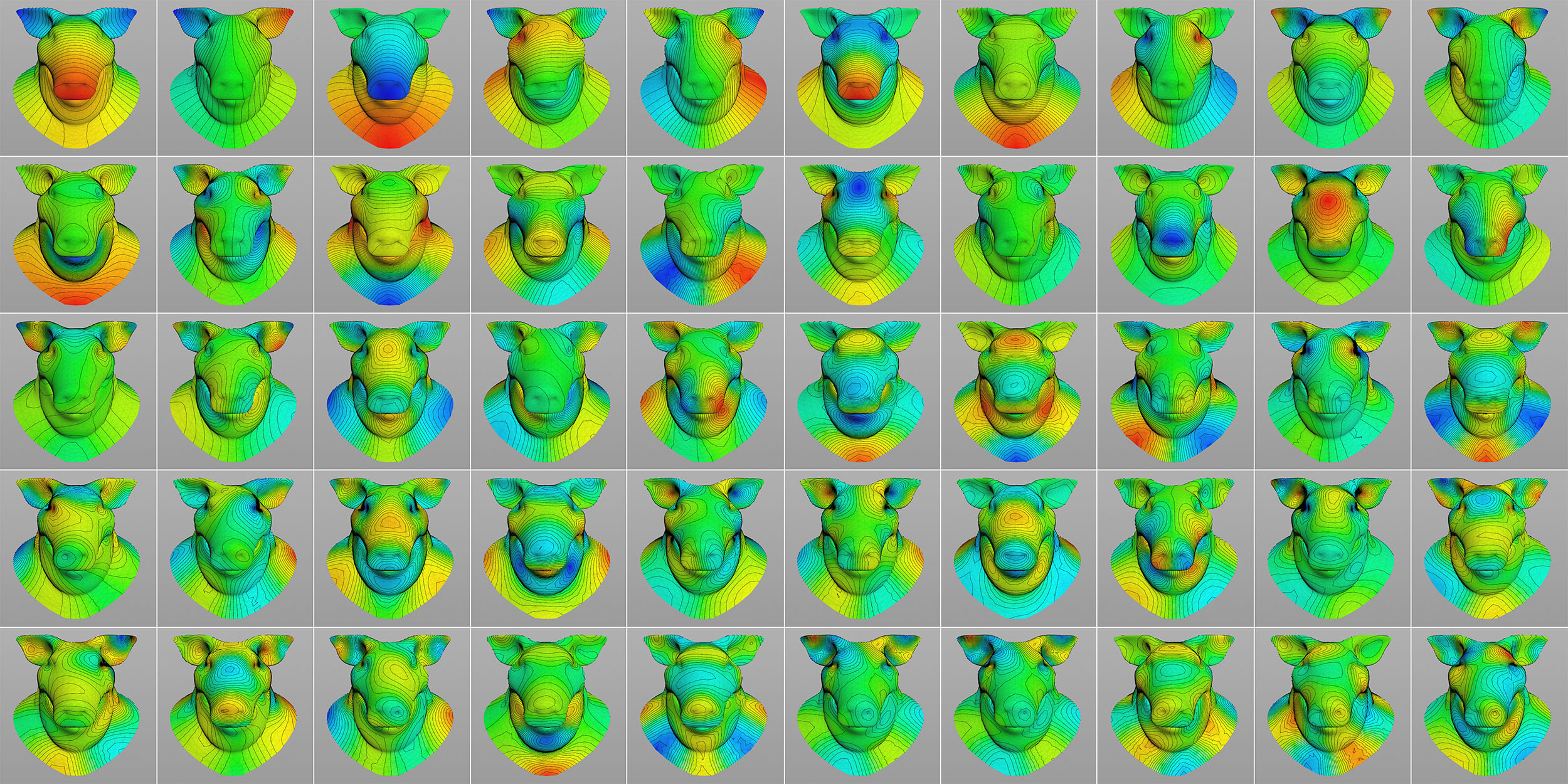
Eigenvectors 1-50
By projecting the point coordinates onto the eigenvectors we can transform the geometry to the corresponding eigenspace. Similar to the Discrete Fourier Transform, the new mapping could then be used for doing various calculations. which are easier to perform in the spectral domain, such as clustering and segmentation.
Eigenvector 3
Eigenvector 6
Eigenvector 8
Eigenvector 10
Eigenvector 15
Eigenvector 30
Eigenvector 50
Eigenvector 1-100
A very important property of eigenvalues and eigenvectors of the Laplace-Beltrami operator is that they are invariant under isometric transformations/deformations. In other words, for two isometric surfaces the eigenvalues and eigenvectors coincide and consequently their eigenvector projection also coincide. Since a character in different poses is usually a near-isometric deformation, eigenfunctions are quite useful for finding non-rigid transformations or for matching different poses. For instance, if we have two characters like in the example below, we can rely on eigenvectors to compute a correspondence matrix and therefore find corresponding points on the two meshes. Subsequently, these points could then be used to match one pose to the other. Now you might ask why do we need eigenvectors for this? Well, if it is the same character in different poses, or more precisely, the same geometry with the same pointcount, this is easy. If it’s not the same geometry, things get much harder. This is typically the case if we are working with 3D scanned models or shapes which have been remeshed like in the example below. The two characters have different pointcounts: The mesh of the left character has 1749 points, the mesh of the right character has 1928 points.
Characters with different pointcounts.
Eigenvectors of the Laplace-Beltrami operator
Corresponding points
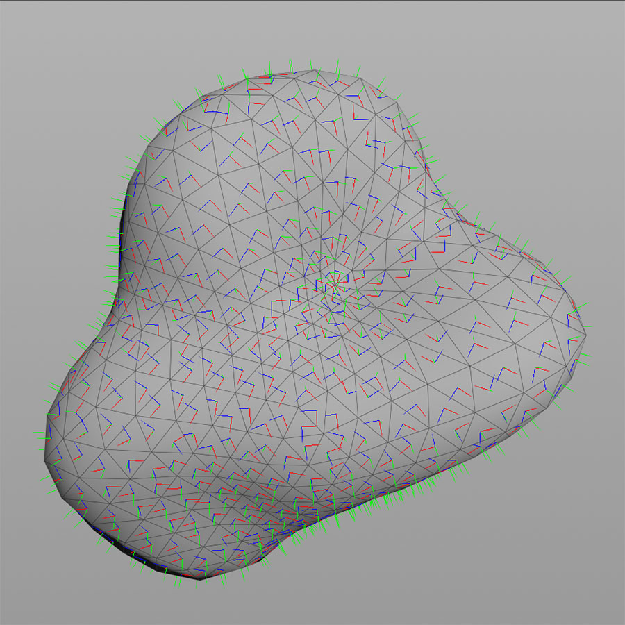
A very useful tool is the Fiedler vector which is the smallest non-zero eigenvector. It is a handy shape descriptor and can be used to compute shape aware tangent vector fields, to align shapes, to compute uvs, for remeshing and many other things. The images below show that isolines based on the Fiedler vector are nicely following the shape of different meshes.
If you ever had to compute an object oriented bounding box by yourself you probably came across the term covariance matrix. Well, this is no accident since covariance matrices are widely used in computer graphics for many different applications such as data fitting, rigid transformation, point cloud smoothing and many more. A covariance matrix is a N x N matrix basically measuring the variance of data in N dimensions. In case of Houdini’s three-dimensional coordinate system it’s therefore a symmetric 3 x 3 matrix capturing the variance in its diagonal and the covariance in its off-diagonal. Computing the covariance matrix is fairly easy and could be done efficiently in VEX or Python/Numpy. The interesting thing about the matrix is that it represents the variance and the covariance of the data. In other words, it describes the “shape” of the data. This means that we can, for example, find the direction of the largest variance measured from the centroid, which consequently is the largest dimension of the data. This is done by decomposing the matrix into its eigenvalues and eigenvectors. In case we are working with a 3 x 3 covariance matrix we get three eigenvectors. The eigenvector with the largest eigenvalue is the vector pointing into the direction of the largest variance. The eigenvector with the smallest eigenvalue is orthogonal to the largest eigenvector and, of course, pointing into the direction of the smallest variance.
Pointcloud in three-dimensional space
Best fitting line representing eigenvector with largest eigenvalue
Best fitting plane representing eigenvector with smallest eigenvalue
Finding the eigenvectors for a small matrix is quite easy and could be done, for example, by using singular value decomposition (SVD) in Numpy. In VEX we don’t have such a function but we could implement a (inverse) power iteration algorithm to find the largest and/or smallest eigenvector. The missing third eigenvector is then computed simply by talking the cross product of the other two already known vectors.
Finding these eigenvectors is quite useful for many applications. For instance, if we need to compute object oriented bounding boxes for each polygon of a mesh. We could do this by building the covariance matrix for the points of each polygon and then searching for the largest eigenvector. Together with the normal, which is the smallest eigenvector, we finally can compute the oriented bounding box. Another useful application of the covariance matrix is the computation of point normals for a point cloud. In this case we need to find the smallest eigenvector, which represents the best fitting plane and thus the normal of the point. Building the covariance matrix is also important if we want to find the rigid transformation from one object to another. All these are just a few examples and to cut a long story short, covariance matrices are quite useful and definitely worth looking into.
Local coordinates based on eigenvectors of covariance matrix
Some time ago I wrote a blog post about geodesics and different methods how they could be computed in Houdini. Geodesic distances are great since they represent the distance, or more precisely, the shortest distance between points on a surface. While this is an important property and useful for many things we might run into a situation in which other properties are even more important, for instance smoothness. This might be the case if we want to generate a smooth vector field based on the distance or if we are working on meshes with holes for example. However, a nice solution to these problems is to compute biharmonic distances instead of geodesic distances. Biharmonic distance is not necessarily the true distance between points on a surface but it is smooth and globally shape-aware.
Biharmonic distance field
Geodesic distance field
Gradient of biharmonic distance
Gradient of geodesic distance
Contrary to geodesic distance, the biharmonic distance is not computed directly on the surface but on the eigenvectors of the laplacian. Basically it’s the average distance between pairwise points projected onto incrementally increasing eigenvectors. The general accuracy is therefore highly dependent on the number of computed eigenvectors – the more the better. If we need to get exact distances we have to compute all eigenvectors or in other words, we need to perform the computationally rather expensive full eigendecomposition of the laplacian. For a sufficient approximation however, we usually can get away with the first 20-100 eigenvectors depending on mesh density and shape. For the implementation in Houdini I’m using Spectra and Eigen together with the HDK. Even though it’s quite fast to perform the eigenvalue/eigenvector decomposition, the computation of geodesic distances is of course much faster, especially on large meshes.